Whole genome tracks

Show where a region sits on its chromosome, or lay every sequence of an assembly end to end so the other tracks can be drawn across all of them at once.

The Rust snippets use ?, so they belong in a function that returns Result<(), Box<dyn std::error::Error>>, and names such as hits stand for data you already hold. To choose a track by its picture, start from the gallery.

IdeogramTrack

The whole chromosome drawn end to end across the plotting area, banded where a cytogenetic table exists, with a marker on the part the tracks below are showing. It answers where the region is.

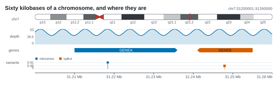
Rust	.add_ideogram(length, bands) on plot(); IdeogramTrack::new(length, bands), IdeogramTrack::bare(length)
Command line	--ideogram FILE, with --height
Reads	a UCSC cytoBand table, the rows for the region's sequence (read::interval::cytoband)

RustCommand line

use karyon::{plot, read};

let text = std::fs::read_to_string("cytoBand.txt")?;
let (length, bands) = read::interval::cytoband(&text, "chr7")?;

plot("chr7:31,200,001-31,260,000")?
    .add_ideogram(length, bands)
    .label("chr7")
    .save("ideogram.svg")?;

karyon chr7:31,200,001-31,260,000 --ideogram cytoBand.txt --label chr7 -o ideogram.svg

Options

Method	What it does	Default
.label("chr7")	Names the track in the left gutter (--label)	none
.height(28.0)	Band height in pixels (--height)	22
.centromere_color("#7f3c8d")	Colour of the centromere	#b03a2e
.outline("#1b1f23")	Colour of the chromosome outline	theme muted grey
.marker_color("#0072b2")	Colour of the marker for the region on display	#d7263d, a red
.show_marker(false)	Shows or hides that marker	shown
.highlight(759_806, 763_325)	Marks another span instead of the region on display	the region
.show_band_names(true)	Draws band names under the chromosome, where they fit	hidden

Notes

This is the one track that draws the whole sequence rather than the region on display, on purpose: a track showing only the region could not say where the region is, since it would be a picture of the window drawn inside the window. Its x is still a genomic coordinate, but not the figure's. A point halfway across the band is halfway along the chromosome, so nothing in it is to be read against a ruler below it.

The marker has a minimum width, because ten kilobases of a five megabase chromosome is a fraction of a pixel, and a pointer too thin to see answers nothing. highlight marks something the figure does not otherwise draw, such as a whole gene while the tracks below show one exon of it.

A cytoBand row converts through Stain::from_name using UCSC's own stain names, and an unknown stain becomes the palest band rather than an invented dark one. The shades are mixed from the theme's ink and page, so a dark figure gets a dark ladder, and the centromere is drawn as a waist rather than as one more band. The chromosome's length is the highest end the table gives for it. Band names are off by default, and the command line has no flag to turn them on.

Most sequences have no cytogenetics to speak of: plasmids, organelle genomes, viruses, draft assemblies and bacterial chromosomes among them. IdeogramTrack::bare(length) gives an outline with the marker, which still answers the only question the track is asked.

GenomeTrack

The sequences of a Genome laid end to end as alternating named blocks: the bar under a figure drawn across a whole assembly, showing which sequence a mark is on and where each one ends.

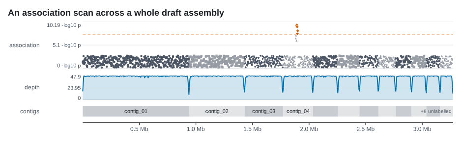
Rust	.add_genome(genome) on plot(); GenomeTrack::new(genome)
Command line	none: library only, as the axis it labels is built in Rust with Genome
Reads	nothing from a file; build a Genome from sequence names and lengths

Rust

use karyon::{Association, Genome, Plot};

let genome = Genome::new([("chr1", 900_000u64), ("chr2", 600_000), ("chr3", 500_000)]);

// hits: Vec<(String, u64, f64)>, a sequence name, a 0-based position on it, and -log10(p)
let (mapped, unplaced) = genome.map(hits);
println!("{unplaced} hits named no sequence of this genome, or ran past its end");
let points: Vec<Association> = mapped
    .into_iter()
    .map(|(at, value)| Association::new(at, value))
    .collect();

Plot::over(genome.region())
    .remove_region_label()
    .remove_axis()
    .add_manhattan(points)
    .label("association")
    .adjust(|track| track.bands(genome.boundaries()))
    .add_genome(genome)
    .label("sequences")
    .save("genome-wide.svg")?;

Options

Method	What it does	Default
.label("sequences")	Names the track in the left gutter	none
.height(28.0)	Band height in pixels	22
.color("#0072b2")	The colour the two alternating shades are mixed from	theme muted grey
.show_names(false)	Shows or hides the sequence names	shown
.min_name_width(8.0)	How much room a name needs before it is written, in pixels	4

Notes

A figure is one region on one sequence, which is right for a locus and wrong for an assembly. A Genome lays the sequences end to end and genome.region() is the one region covering them all, so every other track draws across the lot unchanged. Positions cross onto that axis with Genome::at(name, position) or Genome::map, and both refuse to guess: a name the genome does not have, or a position past the end of its sequence, is dropped and counted rather than drawn somewhere plausible inside the next sequence.

What the track refuses to be is a ruler. A ruler of global coordinates under a concatenated genome measures a coordinate system nothing else uses, since nobody quotes a position as "1,437,902 bases into the assembly", so this track names the sequences and marks where each ends. plot() still appends its own ruler of global coordinates, as the figure above shows, and .remove_axis() leaves it out.

An assembly of two hundred contigs has two hundred names and room for perhaps twelve, so the names that do not fit are left out rather than overprinted, and how many went unwritten is printed inside the bar. named(&scale, &theme) gives that count before anything is drawn. The blocks alternate between two shades of one hue rather than taking a colour each, because what a reader needs from the bar is the joins, and the hues in the figure are left to the tracks carrying data.

For a genome-wide association figure, pass genome.boundaries() to ManhattanTrack bands so its shading changes where each sequence starts. Genome::gap(bases) puts blank axis between the sequences when you want the joins visible without the bar.