Variation tracks¶

Draw how samples differ from a reference and from each other: point calls, structural calls, copy number, variable sites, genotype matrices, association scans and site-wise selection.

The Rust snippets use ?, so they belong in a function that returns Result<(), Box<dyn std::error::Error>>, and names such as tree stand for data you already hold. To choose a track by its picture, start from the gallery.

VariantTrack¶

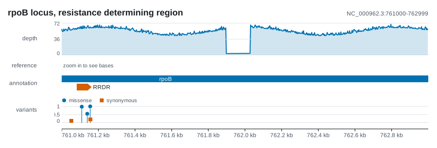
Point events along the sequence, drawn as lollipops whose height is a value, or as plain ticks once they are too dense for heads: SNPs, indels, insertion sites, peaks. Colour and the legend follow each call's category.

Variant calls in rpoB drawn as lollipops whose height is the allele fraction and whose colour is missense or synonymous, under the gene model


Rust	`.add_variants(variants)` on `plot()`; `VariantTrack::new(variants)`
Command line	`--variants FILE`, with `--style`, `--height`
Reads	VCF: `AF` as the value, and the `ANN` or `BCSQ` consequence, or the shape of the call, as the category (`read::point::variants`)

RustCommand line

use karyon::{plot, Variant};

plot("NC_000962.3:761,001-763,000")?
    .add_variants(vec![
        Variant::new(761_108).value(0.98).category("missense"),
        Variant::new(761_154).value(1.00).category("missense"),
        Variant::new(761_155).value(0.21).category("synonymous"),
    ])
    .label("variants")
    .adjust(|track| track.max(1.0))
    .save("variants.svg")?;

karyon NC_000962.3:761,001-763,000 --variants calls.vcf --label variants -o calls.svg

Options¶

Method	What it does	Default
`.label("variants")`	Names the track in the left gutter (`--label`)	none
`.height(70.0)`	Band height in pixels (`--height`)	`55`
`.style(VariantStyle::Tick)`	`Lollipop` or `Tick` (`--style lollipop` or `tick`)	`Lollipop`
`.radius(3.0)`	Radius of a lollipop head	`4`
`.max(1.0)`	Pins the value that reaches the top of the band	the largest value on screen
`.axis(QuantitativeAxis::new())`	Replaces the value axis	automatic
`.show_legend(false)`	Shows or hides the category legend	shown
`.show_scale(false)`	Shows or hides the value axis	shown
`.axis_title("AF")`	What the stems measure, under the track's name while the axis is drawn (set by the command line)	none
`.color("#555555")`	Colour of variants without a category	theme accent

Notes¶

Categories take palette colours in order of first appearance, not by hash, so the same list always gives the same figure. That determinism is the refusal: a figure that recolours itself when a sample is added is not one you can put in a paper. Sorting the same variants differently hands out different colours, so two figures that must agree on what red means need their variants in one order.

A variant with no value gets a full-height stem, which is right when there is no quantity to show. Ticks ignore values altogether, and the value axis is drawn only when the stems are measuring something. Pin max whenever two panels carry the same quantity.

Lollipops read well up to a few hundred calls; past that the heads smear, and Tick is the answer. Ticks carry no tooltip, since a mark nobody can isolate is not worth naming.

From VCF, POS becomes POS - 1, a row with several alternates gives one call per allele, and a call with no AF has no value, and stands full height. Rows without an alternate allele, most of a gVCF, are skipped.

StructuralTrack¶

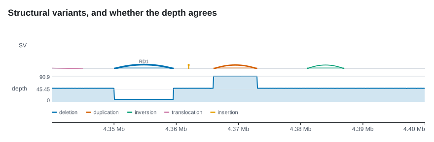
Structural variant calls as arcs between their two breakpoints, springing from the axis at both ends, higher the further apart the ends are and heavier the more reads support them. Use it with a CoverageTrack underneath.

Five structural variant calls drawn as arcs between their breakpoints: a deletion, a duplication, an inversion, an insertion, and a translocation whose far end leaves the frame. Underneath, a depth profile that drops to nothing under the deletion and steps up under the duplication


Rust	`.add_structural(variants)` on `plot()`; `StructuralTrack::new(variants)`
Command line	`--structural FILE`, with `--no-names`, `--height`
Reads	VCF with symbolic alleles or `SVTYPE`, breakend pairs read from the `ALT` (`read::structural::variants`)

RustCommand line

use karyon::{plot, StructuralVariant, SvKind};

// depth: Vec<f64> from 0-based 4,330,000
plot("NC_000962.3:4,340,001-4,400,000")?
    .add_structural(vec![
        StructuralVariant::new(4_352_000, 4_356_000, SvKind::Deletion).support(31),
        StructuralVariant::new(4_370_000, 4_376_000, SvKind::Duplication).support(12),
        StructuralVariant::new(4_381_000, 4_390_000, SvKind::Inversion).name("inv1"),
    ])
    .label("SV")
    .add_coverage_at(4_330_000, depth)
    .label("depth")
    .save("sv.svg")?;

karyon NC_000962.3:4,340,001-4,400,000 \
  --structural sv.vcf --label SV \
  --coverage sv-depth.bedgraph --label depth \
  -o sv.svg

Options¶

Method	What it does	Default
`.label("SV")`	Names the track in the left gutter (`--label`)	none
`.height(120.0)`	Band height; the widest arc in view uses all of it but the line its name needs (`--height`)	`90`
`.color(SvKind::Deletion, "#d55e00")`	Colour of one kind of call	a palette colour per kind
`.stroke(1.0, 4.0)`	Arc weight at no support and at full support	`1.0` to `3.4`
`.saturating_support(50)`	Read count at which an arc is drawn at full weight	`30`
`.show_footprints(false)`	Shows or hides the bar along the axis under calls that cover sequence	shown
`.show_names(false)`	Shows or hides names over the arcs (`--no-names`)	shown

Notes¶

The arc is the point. A structural variant is a statement that two positions belong together: the two ends of a deletion, the source and destination of a duplication. A VariantTrack draws one point per call and cannot say that, and a bar spanning the event says only that something happened in the middle, which is usually the one place nothing happened.

Height is an ordering within one view, never a length and never comparable across two. The widest call lying wholly inside the view reaches the top of the band, a call wider than that (which can only be one leaving the view) reaches the top too, and the rest follow the square root of their span. So a translocation off to the side does not press the arcs you are looking at flat, and panning or zooming rescales them.

Half of reading a call is whether the depth agrees: a deletion with no drop under it and a duplication with no rise are calls to argue with. An insertion has one breakpoint and no footprint; a translocation joins two places rather than covering what lies between them.

The VCF reader takes nothing off POS for a symbolic allele, because the specification puts POS on the base before the event. The span comes from SVLEN (its absolute value), else END, else the length of REF, and a record stating none of them is refused rather than drawn one base wide. Of the two records of a breakend pair, only one becomes an arc.

CopyNumberTrack¶

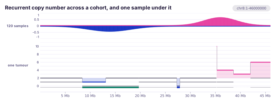
Segmented copy number on a ladder of whole copies, with a lane along the foot marking where one allele was lost. Every called segment is a mark, and only a segment nobody called is blank.

Above, the share of a cohort with a gain or a loss along one chromosome arm; below, one tumour's segments on a ladder of whole copies, with its loss of heterozygosity marked along the foot


Rust	`.add_copy_number(segments, ploidy)` on `plot()`; `CopyNumberTrack::at_ploidy(segments, ploidy)`, `CopyNumberTrack::diploid(segments)`, `CopyNumberTrack::haploid(segments)`
Command line	`--copy-number FILE --ploidy COPIES`, with `--sample`, `--height`
Reads	a segment table with a header: CNVkit `.cns`, ASCAT, or `.seg` (`read::segments::copy_numbers`)

RustCommand line

use karyon::{plot, CopyNumberSegment};

let segments = vec![
    CopyNumberSegment::allelic(0, 12_000_000, 1.0, 1.0),
    CopyNumberSegment::allelic(12_000_000, 20_000_000, 2.0, 0.0), // copy-neutral LOH
    CopyNumberSegment::total(20_000_000, 26_000_000, 1.0),
    CopyNumberSegment::allelic(26_000_000, 38_000_000, 2.0, 1.0),
];

plot("chr8:1-46,000,000")?
    .add_copy_number(segments, 2.0)
    .label("copy number")
    .save("copy-number.svg")?;

karyon chr8:1-46,000,000 --copy-number tumour.cns --ploidy 2 --label 'copy number' -o cn.svg

Options¶

Method	What it does	Default
`.label("copy number")`	Names the track in the left gutter (`--label`)	none
`.height(100.0)`	Band height in pixels (`--height`)	`74`
`.cap(8.0)`	Pins the top rung of the ladder, taken literally	at least two copies above the ploidy
`.colors(gain, loss, neutral)`	Inks for gain, loss and the balanced state	from the theme
`.loh_color("#6a3d9a")`	Ink of the lost-heterozygosity mark	from the theme
`.show_scale(false)`	Shows or hides the copy scale	shown
`.show_alleles(false)`	Shows or hides the allele lane along the foot	shown

Notes¶

Where balanced sits has no default, in at_ploidy or on the command line, where --ploidy is required. The crate does not know what it is drawing, and a rule in the wrong place does not merely mis-scale the ladder: it swaps every gain for a loss. diploid and haploid say it for you.

A level is a bar drawn at the level, not a fill from a line to it. A window track fills from its baseline, so a segment called exactly at the ploidy draws nothing, and a balanced segment is most of a genome: its quiet arms would look the same as arms nobody called. That is why this is not a WindowTrack.

A minor allele of nought with copies still present is a finding, so it must not look like the absence of one. CopyNumberSegment::allelic carries both alleles; CopyNumberSegment::total carries a total and says nothing about them, and its minor() is None rather than nought. Copy-neutral loss of heterozygosity puts the total bar exactly on the balanced rule, and the lane along the foot is what shows it.

Copies are continuous, since subclonal and purity-adjusted calls are fractional; the rungs are at whole copies because that is where the interpretable states are. Nothing is averaged: every segment is drawn at its own level, a pixel wide where it is narrower, with a hairline joining the extremes in each column, and nothing is drawn between two segments.

A log2 ratio from a .seg or .cns becomes copies as ploidy * 2^log2, and a called copy number is used where the table has one. --sample picks one sample from a table holding several.

SnpTrack¶

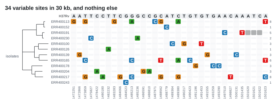
The variable columns of an alignment and nothing else, spaced evenly, one row per sample, each column labelled with its own position. Put a phylogeny beside it and a clade's shared substitutions line up into a block.

A phylogeny, three strips of sample metadata and a panel of thirty-four variable sites across twelve isolates, each column labelled with its position


Rust	`.add_snps(names, sites)` on `plot()`; `SnpTrack::new(names, sites)`, `SnpTrack::from_alignment(reference, &rows)`
Command line	`--snps FILE`, with `--compare-to`, `--no-counts`, `--row-height`, `--max-rows`, `--no-names`, `--traits`, `--columns`
Reads	aligned FASTA, compared against its first record unless `--compare-to` names another (`read::seq::alignment`)

RustCommand line

use karyon::{Plot, Region, SnpTrack};

// rows: Vec<MsaSequence>, aligned, with the reference as row 0; tree: Tree
let panel = SnpTrack::from_alignment(0, &rows).tree(tree).label("isolates");
let sites = panel.sites().len() as u64;

Plot::over(Region::new("sites", 0, sites)?)
    .remove_region_label()
    .add_track(panel)
    .save("snps.svg")?;

karyon --snps isolates.fa --compare-to H37Rv --label isolates \
  -o snps.svg

Options¶

Method	What it does	Default
`.label("isolates")`	Names the track in the left gutter (`--label`)	none
`.row_height(16.0)`	Height of one row (`--row-height`)	`15`
`.row_gap(3.0)`	Gap between rows	`2`
`.offset(1_472_000)`	Shifts every site position, for an alignment that starts away from zero	`0`
`.reference_name("H37Rv")`	Names the reference row	`"reference"`, or the row's own name from `from_alignment`
`.show_reference(false)`	Shows or hides the reference row along the top	shown
`.show_names(false)`	Shows or hides sample names (`--no-names`)	shown
`.show_positions(false)`	Shows or hides the position under each column	shown
`.show_counts(false)`	Shows or hides each row's count of differences (`--no-counts`)	shown
`.zebra(false)`	Shows or hides the alternating column tint	shown
`.max_rows(Some(100))`	Caps the sample rows drawn; `None` lifts the cap (`--max-rows`)	`Some(40)`
`.match_color("#e5e7eb")`	Colour of a cell that matches the reference	from the theme
`.tree(tree)`	Draws a phylogeny beside the panel and sorts the rows to match it	none
`.tree_width(120.0)`	Width of the tree strip in pixels	`90`
`.tree_shape(TreeShape::Cladogram)`	Phylogram or cladogram for that tree	`Phylogram`
`.traits(traits)`	Metadata columns between the names and the panel (`--traits`, `--columns`)	none

Notes¶

An alignment of close relatives is almost all agreement: thirty kilobases carrying thirty-four differences would spend 99.9% of its pixels on the part that says nothing. Dropping the invariant columns turns a smear into legible columns. A cell that matches the reference is a quiet bar, alternate columns are tinted so the eye can cross a wide panel, and each row carries its count of differences on the right.

The price is the x axis. Two neighbouring columns may be nine bases or nine kilobases apart, and nothing about the spacing says which, so each column carries its own position turned on end, counted from one like a ruler's, and a ruler does not belong under the panel. The region is the site index space, Region::new("sites", 0, 34) for thirty-four sites. The panel answers false to Track::on_coordinates, so plot() and the command line append no ruler for it; a figure that also holds a track on the coordinates keeps the ruler that track is read against.

A panel with more sites than pixels, the whole genomes of an outbreak say, is drawn a pixel at a time once a column would be narrower than a pixel and a half. Each pixel of a row is shaded by the share of the sites under it that differ from the reference, in eight steps from the colour of an agreement to the colour of a difference, and the key says so. A pixel with any difference in it takes at least the first step, so one difference among forty sites is not drawn as agreement. The positions, the strip under the panel that holds them and the column tint go, since there is no room for them, and each row's tooltip counts its differences. Thirty thousand sites of forty samples were an SVG of 124 MB drawn a cell at a time, which no viewer opens, and are about a megabyte this way.

from_alignment(reference, &rows) keeps a column when any row disagrees with the reference row, gaps included, since a deletion is an observation too. Positions are alignment columns, counted from 0 and labelled from 1; offset moves them to where the alignment starts.

tree sorts the rows by descent, so a clade's shared substitutions line up into a block. Rows are matched to leaves by name, and a sample the tree does not mention keeps its place at the bottom rather than vanishing: a row silently dropped from a figure is worse than a row out of order. The same tree beside a MatrixTrack, MsaTrack or DomainTrack sorts it the same way.

MatrixTrack¶

One row per sample, one column per site, and a cell saying what that sample had there. The columns sit at their real coordinates, so the matrix shares the axis with whatever is stacked above it: a genotype matrix from a VCF, or a presence and absence matrix of genes.

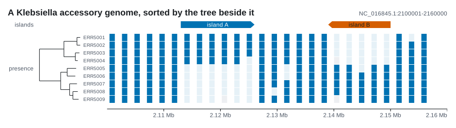
A presence and absence matrix of accessory genes across nine Klebsiella isolates, with the phylogeny beside it ordering the rows so the accessory islands come out as solid rectangles


Rust	`.add_matrix(sites, rows)` on `plot()`; `MatrixTrack::new(sites, rows)`, and `MatrixTrack::windows(windows, rows)` for a column per window
Command line	`--matrix FILE` for sites, `--heatmap FILE` for windows, with `--with-tree`, `--row-height`, `--no-names`, `--traits`, `--columns`; `--relative` and `--center` after `--heatmap`
Reads	a table with 1-based site positions across the header and one row per sample (`read::table::matrix`); or windows as `bedtools unionbedg` writes them, a sequence, a start and an end, then a column per sample, or in the long form, a sample and its value to a row (`read::table::windows`). An empty cell, `.` or `NA` is missing

RustCommand line

use karyon::{plot, CellScale, MatrixRow};

let sites = vec![759_949, 760_399, 761_154];
let rows = vec![
    MatrixRow::new("ERR001", vec![1.0, 0.0, 1.0]),
    MatrixRow::new("ERR002", vec![0.0, f64::NAN, 1.0]), // NaN: not typed here
];

// tree: a Tree whose leaves are named ERR001 and ERR002
plot("NC_000962.3:759,001-765,000")?
    .add_matrix(sites, rows)
    .label("genotypes")
    .adjust(|track| {
        track
            .scale(CellScale::Sequential { max: Some(1.0), hue: None })
            .tree(tree)
    })
    .save("matrix.svg")?;

karyon NC_000962.3:759,001-765,000 \
  --matrix genotypes.tsv --traits samples.tsv --columns lineage,host \
  --label genotypes -o matrix.svg

Options¶

Method	What it does	Default
`.label("genotypes")`	Names the track in the left gutter (`--label`)	none
`.row_height(14.0)`	Height of one row (`--row-height`)	`11`
`.row_gap(2.0)`	Gap between rows, in the page colour	`1`
`.scale(CellScale::Categorical)`	How a value becomes a colour: a one-hue `Sequential` ramp, `Categorical` palette indices, or `Diverging { center, spread }`, two hues either side of a centre (`--center`, and `--relative` about 1)	`Sequential { max: None, hue: None }`
`.missing_color("#bdbdbd")`	Colour of a missing cell	from the theme
`.min_cell_width(4.0)`	Narrowest a cell is drawn, in pixels	`3`
`.show_row_names(false)`	Shows or hides sample names (`--no-names`)	shown
`.tree(tree)`	Draws a phylogeny beside the rows and sorts them to match it	none
`.tree_width(120.0)`	Width of the tree strip in pixels	`90`
`.tree_shape(TreeShape::Cladogram)`	Phylogram or cladogram for that tree	`Phylogram`
`.traits(traits)`	Metadata columns between the names and the cells (`--traits`, `--columns`)	none
`.unit("×")`	Written after the two numbers at the ends of the key	none

Notes¶

Three things must look different: a sample that does not carry the allele, a sample that was never typed, and a stretch with no site at all. So the sequential ramp starts a step off the page colour rather than on it, and missing data has its own grey: f64::NAN is missing, and zero is a genotype. Sequential is one hue from light to dark, because two hues would imply a meaningful middle; Categorical reads the value as an index into the palette, for genotypes that name rather than measure.

A cell's width is a floor, min_cell_width, so it says nothing about how much sequence it covers. A matrix of windows is the other kind: MatrixTrack::windows takes a 0-based, half-open span for each column, and each cell covers exactly its window, as the depth of forty samples in windows of 100 kb does on the command line with --heatmap. There --relative divides each sample by its own median first, so 1× is its usual value and a sample sequenced deeper is not a darker row from end to end.

A sequential ramp is keyed under the figure, from nought to the value it saturates at, which is how a reader learns how deep a dark cell is.

A quantity with a middle that means something is Diverging: the centre is drawn pale, in neither hue, a value below it in the theme's first colour and one above it in the second, as a CopyNumberTrack draws a loss and a gain. With no spread, each side is at full strength at its own furthest value, so depths from nothing to three times the usual run from a full loss at 0× to a full gain at 3×, and the key writes the centre between the two halves of its strip, since the ends are not the same distance from it. --relative reads the depths this way about 1×, where one hue drew a lost stretch nearly as pale as the page.

tree sorts the rows by descent, which is what turns a speckle into rectangles; rows the tree does not name stay at the bottom. Cells never merge, and that is the refusal: six carriers drawn as six cells are six observations, and one rectangle covering a clade is a different claim, made by a CladeTrack.

ManhattanTrack¶

Association statistics: one point per test, height by significance, a line where significance starts, and the hits above it coloured and ringed. A real signal stacks neighbouring markers into a tower.

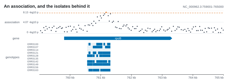
A Manhattan plot with a tower crossing the significance line, the gene underneath it, and a genotype matrix showing which isolates carry the haplotype


Rust	`.add_manhattan(points)` on `plot()`; `ManhattanTrack::new(points)`
Command line	`--manhattan FILE`, with `--threshold`, `--ld`, `--with-recombination`, `--height`
Reads	two columns, position and value, or three with a sequence name first; 1-based positions, and the value drawn as given (`read::point::associations`)

RustCommand line

use karyon::{plot, Association};

// hits: Vec<(u64, f64)>, a 0-based position and a p-value for each test
let points: Vec<Association> = hits
    .iter()
    .map(|&(pos, p)| Association::from_p_value(pos, p))
    .collect();

plot("NC_000962.3:759,001-765,000")?
    .add_manhattan(points)
    .label("association")
    .adjust(|track| track.p_value_threshold(1e-6).axis_title("-log10 p"))
    .save("scan.svg")?;

karyon NC_000962.3:759,001-765,000 \
  --manhattan scan.tsv --threshold 5 --label association -o scan.svg

Options¶

Method	What it does	Default
`.label("association")`	Names the track in the left gutter (`--label`)	none
`.height(120.0)`	Band height in pixels (`--height`)	`90`
`.threshold(6.0)`	Draws a line at this value, labelled with it, and colours what reaches it (`--threshold`, for a file of scores)	none
`.p_value_threshold(1e-6)`	The line at `-log10` of a p-value, labelled `p = 1e-6` (`--threshold`, for a file of p-values)	none
`.genome_wide_threshold()`	The line at `-log10(5e-8)`, about 7.3, labelled `p = 5e-8` (`--threshold genome-wide`)	none
`.threshold_label("FDR 5%")`	Words on the line in place of its value; `""` for none	the value
`.bands(genome.boundaries())`	Alternates the point colour at each position, for sequences laid end to end	none
`.radius(3.0)`	Radius of a point	`2.2`
`.max(12.0)`	Pins the top of the axis	the tallest point or the threshold, rounded up
`.axis(QuantitativeAxis::new())`	Replaces the value axis	automatic
`.color("#9ca3af")`	Colour of points below the line	theme muted grey
`.significant_color("#d55e00")`	Colour of points at or above it	a palette colour
`.axis_title("-log10 p")`	What the axis measures, under the track's name (set by the command line for a file of p-values)	none
`.unit("x")`	Suffix after the top number, for a unit written as a symbol	none
`.show_scale(false)`	Shows or hides the value axis	shown
`.linkage(lead, r2)`	Colours each point by its r² with the lead variant at `lead`, 0-based, and draws the lead as a diamond with its position over it (`--ld`)	one colour
`.lead_name("rs1234")`	Calls the lead by its name over the diamond and in the key, in place of its position (from the scan's `SNP` or `ID` column, or the `.ld` table's)	its position
`.recombination(rates)`	Lays a recombination rate over the scan as a line, from 0-based half-open `(start, end, cM/Mb)` spans, read off a scale on the right (`--with-recombination`)	none

Notes¶

There is no default threshold, on purpose, and significant() returns nothing until there is one. genome_wide_threshold is a Bonferroni correction for a million independent tests: the convention in human GWAS, and often the wrong number elsewhere, because the right one follows from how many independent tests were really run, and a shorter genome or stronger linkage leaves far fewer than a million.

Association::from_p_value converts a p-value to -log10(p); Association::new plots the value as it is. The command line reads the header: a column named as p-values are, P, pvalue, p_wald and the like, is drawn as -log10 with the axis saying so, and --threshold is then a p-value too; any other column, -log10(p) or another score, is drawn as written with a --threshold in the same units. The association table has the whole rule. In Rust, name what the axis measures with axis_title.

Points are small on purpose, since the plot is read as a texture with towers in it, and a hit gets a ring rather than a bigger disc.

linkage draws a peak the way LocusZoom does: every point coloured from grey to the accent by its r² with the lead, and the lead a diamond with its name or its position over it, both keyed under the figure. recombination lays the rate under the points, as LocusZoom does too, on a scale of its own on the right with its unit after the highest number: a peak ends where the haplotypes it rides on break up, at a hotspot, so the two are read against each other. The figure makes room for that scale on the right of every track, so the bands still end together. A tower beside the peak whose points stay grey is another signal rather than the same one. A point whose linkage is not known is a paler grey than an r² of nought. On the command line --ld names PLINK's table of the lead against its neighbours; the lead is the variant in every row, or, in a table of every pair, the strongest variant of the scan that the table names.

The x axis is genomic, so this draws one sequence or one region of one. For a scan across a whole genome, build the figure over a Genome, pass Genome::boundaries to bands so the shading changes where each sequence starts, and put a GenomeTrack under it.

PairTrack¶

Pairs of places and a value between them: linkage between variants, contacts between the bins of a chromosome, epistasis between sites, loops. A triangle under the axis where most places were measured against their neighbours, and arcs where a few pairs join places far apart.

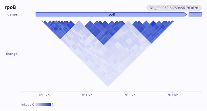
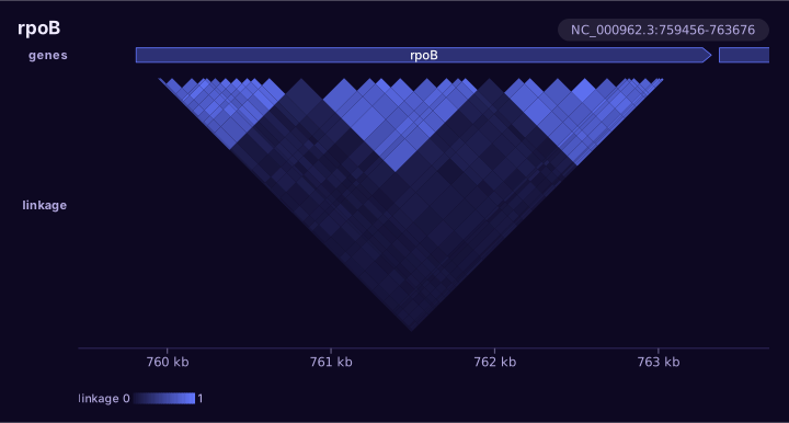
A gene with thirty-six variants under it, and under them a triangle in which each pair of variants is a cell coloured by its linkage: three dark triangles where variants are inherited together


Rust	`.add_pairs(pairs)` on `plot()`; `PairTrack::new(pairs)`
Command line	`--pairs FILE`, or a `.ld` or `.bedpe` named on its own, with `--style`, `--threshold`, `--log`, `--color`, `--height`
Reads	PLINK's `.ld`, BEDPE, or a table headed `pos1`, `pos2` and a value (`read::pairs::pairs`)

RustCommand line

use karyon::{plot, Pair, PairStyle};

// Two variants in strong linkage and a third in weak linkage with both.
let pairs = vec![
    Pair::new(760_101, 760_480, 0.93),
    Pair::new(760_101, 761_900, 0.08),
    Pair::new(760_480, 761_900, 0.11),
];

plot("NC_000962.3:759,807-763,325")?
    .add_pairs(pairs)
    .label("r²")
    .adjust(|track| track.ceiling(1.0).style(PairStyle::Triangle))
    .save("linkage.svg")?;

karyon rpoB genes.gff3 linkage.ld -o linkage.svg

Options¶

Method	What it does	Default
`.label("r²")`	Names the track in the left gutter (`--label`)	none
`.style(PairStyle::Arcs)`	`Triangle` or `Arcs` (`--style triangle`, `--style arcs`)	`Triangle`; on the command line, `PairStyle::for_pairs`
`.height(200.0)`	Band height in pixels (`--height`)	a triangle as deep as its widest pair, up to `240`; arcs `90`
`.ceiling(1.0)`	The value the ramp saturates at	the largest value drawn; `1` on the command line for an r², r or D'
`.threshold(0.2)`	Draws only the pairs at or above this value (`--threshold`)	every pair
`.log_scale(true)`	Colours on a log scale, as a contact map is read (`--log`)	linear
`.color("#d55e00")`	The hue at the top of the ramp (`--color`)	theme accent

Notes¶

A pair is two stretches, Pair::spans for two bins or two anchors, or two single bases, Pair::new for two variants. In a triangle each pair is a cell under the point half way between its places, as deep as they are far apart, so a block of variants inherited together is a dark triangle under the stretch it covers. A single base owns the stretch from half way to the place before it to half way to the one after, so the cells tile the triangle whatever the spacing, and each still sits under its own place. The triangle is squeezed to its band where the widest pair is deeper than it, and never stretched.

PairStyle::for_pairs chooses a triangle where at least half the places are measured against the next place along, as linkage within a window and contact maps are, and arcs where fewer are, as a handful of epistatic sites or loops. The command line draws linkage as a triangle whatever its window left out. A pair with no value, or under the threshold, is not drawn; every drawn pair carries its places, counted from 1, and its value in a tooltip, up to 2,500 cells.

SelectionTrack¶

Site-wise molecular selection in two aligned tiers, so evidence and effect never share one colour: -log10(p) or a posterior probability above, and a signed log2(ω) effect centred on ω = 1 below.

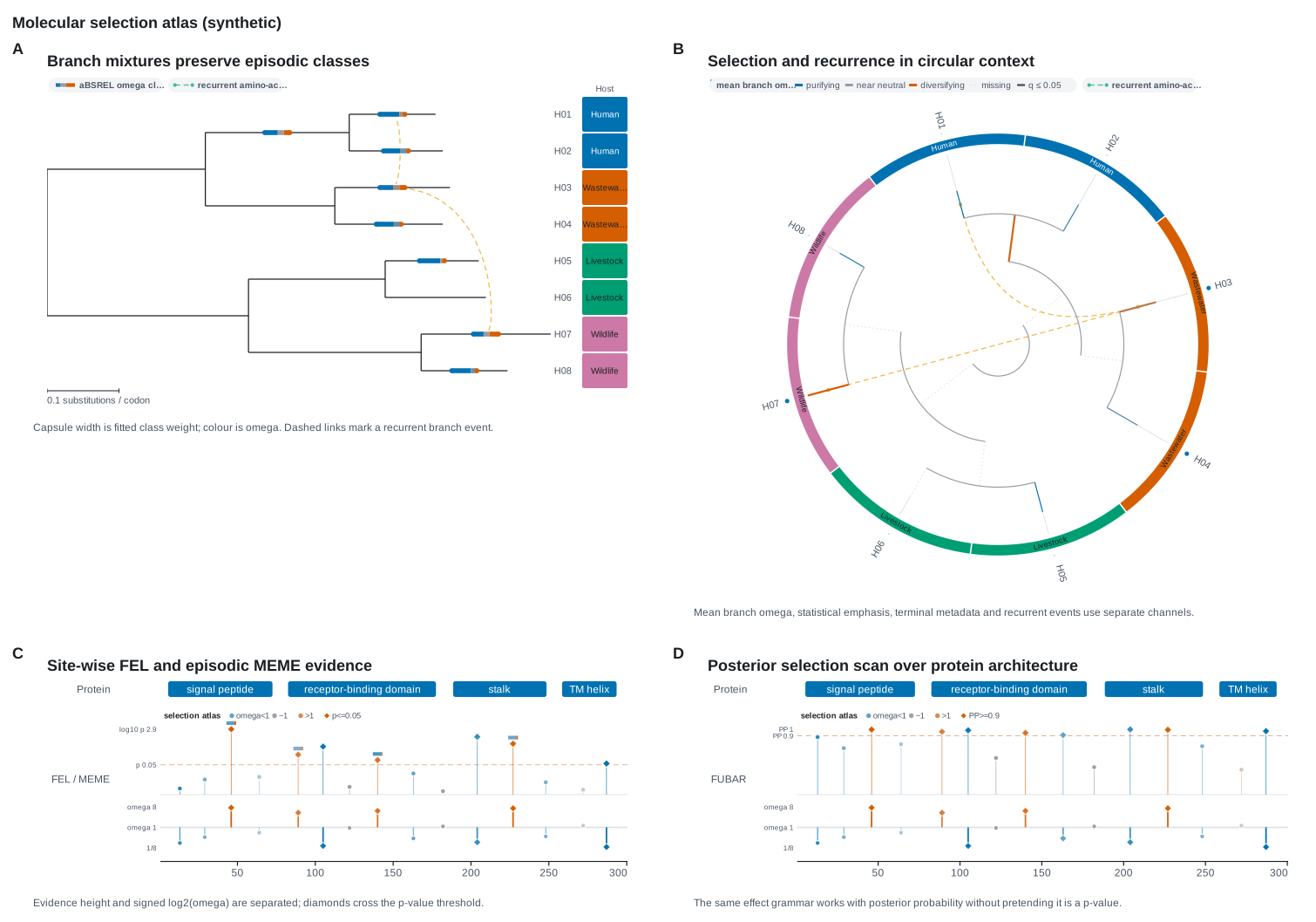
The site-wise panels of a synthetic molecular-selection atlas, with p-value and posterior evidence above signed omega effects and protein domains


Rust	`.add_selection(sites)` on `plot()`; `SelectionTrack::new(sites)`
Command line	`--selection FILE`, with `--threshold`, `--height`
Reads	HyPhy's FEL or MEME CSV as it is, or a table naming its columns: a `site`, the rates as `alpha` and `beta`, `dS` and `dN` or their ratio `omega`, and a `p-value` or a `posterior` (`read::series::selection`)

RustCommand line

use karyon::{plot, SelectionEvidence, SelectionSite};

let sites = vec![
    SelectionSite::new(44)
        .rates(0.18, 1.52)
        .p_value(0.0014)
        .episodic_rates(0.05, 3.8, 0.18),
    SelectionSite::new(103).rates(0.50, 0.07).p_value(0.008),
];

plot("gene:1-300")?
    .add_selection(sites)
    .label("FEL")
    .adjust(|track| {
        track
            .evidence(SelectionEvidence::PValue)
            .p_threshold(0.05)
            .neutral_band(0.85, 1.15)
            .saturation(8.0)
    })
    .save("selection.svg")?;

karyon --selection fel.csv --threshold 0.01 --label FEL -o selection.svg

The table is its own place, and the ruler counts its sites from 1. A table of posteriors only is drawn by its posteriors, and --threshold is then a posterior.

Options¶

Method	What it does	Default
`.label("FEL")`	Names the track in the left gutter	none
`.height(180.0)`	Total height of both tiers, in pixels	`150`
`.evidence(SelectionEvidence::Posterior)`	`PValue` or `Posterior` for the upper tier	`PValue`
`.p_threshold(0.01)`	Significance threshold for p-values (`--threshold`)	`0.05`
`.posterior_threshold(0.95)`	Threshold for posterior probabilities (`--threshold`, for a table of posteriors)	`0.90`
`.neutral_band(0.85, 1.15)`	The ω interval drawn as neutral	`0.90` to `1.10`
`.saturation(4.0)`	The ω at which effect height and colour stop growing	`8`
`.show_evidence(false)`	Shows or hides the evidence tier	shown
`.show_effect(false)`	Shows or hides the effect tier	shown

Notes¶

A site that crosses the threshold is drawn as a larger diamond instead of a small circle. Colour follows the direction of ω and not the evidence, so a significant purifying site keeps the purifying colour.

Missing evidence or rates are left out rather than drawn at nought, the exact values you supplied stay in the tooltips, and an infinite ω from dS = 0 is capped only in the drawn geometry.

SelectionSite::episodic_rates(beta_minus, beta_plus, weight) keeps the two nonsynonymous rate classes of an episodic model and the weight of the positive one; the evidence mark gets a small two-part capsule and the tooltip keeps all three numbers. A class with no ω to draw is counted by undrawable_rate_class_count() rather than painted from an assumed denominator.

The track draws results that were already fitted. It does not fit a codon model or choose a multiple-testing correction. Positions are 0-based genomic coordinates, so domains, variants and a CodonTrack stack above it without relabelling.