Scale

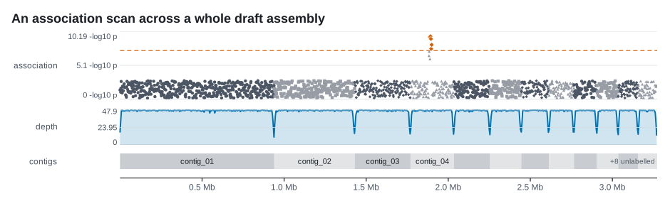
A figure of four megabases is about 900 pixels wide, of which 788 are the plotting area once the left gutter is holding the track labels. One pixel column therefore covers around 5,000 bases, and a track that drew one mark per base would emit four million marks to fill 788 columns. The result would be a file no viewer opens and a picture no reader can tell apart from the correct one.

Every track in the crate is written the other way round: it asks the shared Scale how much sequence a pixel covers and draws at the resolution of the output rather than the resolution of the input. A depth profile over four megabases is then a few thousand marks instead of four million, and the document is a few tens of kilobytes instead of a few tens of megabytes.

The one map

Scale is a linear map from base positions to x coordinates in the output image. One is built per figure, from the region and the plotting area, and every track is handed the same one. That sharing is the whole reason the tracks line up: no track computes its own x.

Method	Answers
x(pos)	left edge of the base at 0-based pos
x_center(pos)	middle of that base
x_at(pos)	left edge of a fractional position
pos_at_x(x)	the inverse: which fractional base sits under a pixel
bp_per_px()	bases covered by one pixel. Above 1, the data must be binned
px_per_bp()	pixels covered by one base. Above roughly 8, there is room for a letter
bounds()	the region on display, 0-based half-open
x0(), width()	the plotting area

let region = Region::new("NC_000962.3", 0, 4_000_000)?;
let scale = Scale::new(&region, 12.0, 872.0);

assert_eq!(scale.bounds(), (0, 4_000_000));
assert!((scale.bp_per_px() - 4_587.2).abs() < 0.05);

bounds() exists because a track is asked how tall it wants to be before it is asked to draw, and some tracks cannot answer without knowing what is on screen. A pileup packs only the reads in view, so its height follows the view.

One point per pixel column

CoverageTrack holds a dense array of values, one per base, which is the shape samtools depth output arrives in. It does not walk that array. It walks the pixel columns of its own band, asks pos_at_x which bases fall under each one, reduces them to a single number, and emits one point:

for column in 0 .. band.w:
    x     = band.x + column
    first = scale.pos_at_x(x)
    last  = scale.pos_at_x(x + 1)
    point = reduce(values[first .. last])

The cost of the output therefore follows the width of the figure, not the length of the input. Four megabases of per-base depth, a four-million-base reference and a coordinate ruler render to a document of about 25 KB, and a test pins that under 100 KB so a change that starts emitting per-base marks fails rather than merely getting slower.

Aggregate, and when it changes the answer

Reducing a column to one number is a choice, and Aggregate makes it explicit because there is no default that is right for every question.

Aggregate	Takes	Use it when
Max	the highest value in the column	hunting for duplications and spikes. The default
Mean	the mean of the column	reading the overall level
Min	the lowest value in the column	hunting for dropouts

The choice stops being cosmetic exactly when the feature you are looking for is narrower than a pixel. Take a 100 base dropout to zero depth in an otherwise flat profile at 60x, drawn across four megabases, where one column holds 4,587 bases:

Aggregate	The column reads	The dropout
Max	60	invisible
Mean	58.7	a 2% dip, which is inside the noise of a real profile
Min	0	the full depth of the hole

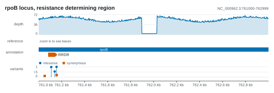
Max is the default because a spike is the commoner thing to be hunting and because it never invents a value the data does not contain. It is also the one that will quietly hide a deletion. The overview figure below uses Aggregate::Min for that reason: at two and a half bases per pixel the dropout is the thing worth not smoothing away.

Two smaller rules go with it. Non-finite values are ignored rather than propagated, so one NaN in a column does not erase the column. And a column with nothing finite in it at all is missing rather than zero: no point is emitted, so a gap in the data reads as a gap rather than as a stretch of zero depth.

What a sequence track does past single base resolution

SequenceTrack climbs three levels of detail, the way a genome browser does:

Resolution	What is drawn
at least 7 px per base	the letter, in the base's colour
down to 0.6 px per base	a coloured block per base, overdrawn by a hair so antialiasing leaves no hairline gaps
below that	the words zoom in to see bases, and nothing else

Both thresholds are settable, with letter_threshold and block_threshold, but the third level is not decoration. A million bases drawn as one-pixel rectangles is a million rectangles; with the hint instead, a figure holding a million-base sequence track comes out under four kilobytes, which is checked by a test.

CodonTrack climbs the same ladder in three steps of its own: translated letters while a codon is wider than the font, alternating cells while a codon is at least 2.5 pixels wide so the partition is still visible, and a plain bar marking the extent of the coding sequence below that, so the codon numbers underneath still have something to belong to.

Every other track that bins

The same discipline appears in a different shape wherever the data are denser than the output.

WindowTrack keeps the lowest and highest value per pixel column rather than one summary, because a signed statistic that swings both ways inside one column has to show both swings: reducing it to a single number would hide the very thing the sign is there to report. Runs of columns carrying the same pair are then emitted as one rectangle, since drawing them one pixel at a time leaves a seam at every join that reads as a bar chart of the wrong bars.

SquiggleTrack draws each column as the range of the samples underneath it, which is the envelope an oscilloscope and an audio editor draw for the same problem. The extremes are honest and the shape between them is not there. Zoom in past the point threshold and the samples are drawn as themselves, with a ringed dot on each.

MsaTrack merges neighbouring cells of the same colour into one rectangle. Most of an alignment agrees with itself, so a row that agrees for eighty columns costs one rectangle rather than eighty. That is the difference between a figure and a file no viewer will open.

PileupTrack only hunts for mismatches once a base is worth at least a fifth of a pixel. Below that, finding one would mean walking every base of every read to draw something nobody can see.

Packing, which is why height takes a scale

Track::height is handed the Scale because some tracks do not have a fixed height. Collisions between features are measured in pixels, not in bases, so how many rows a track needs is a property of the zoom level.

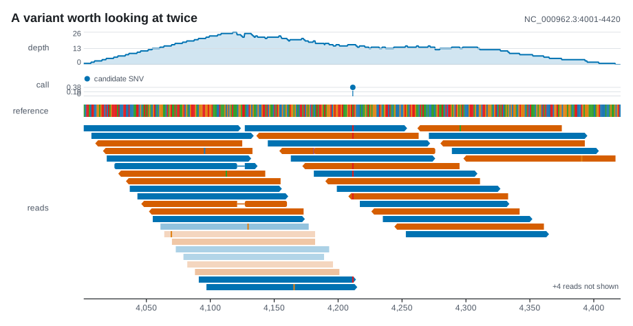
FeatureTrack sorts by start and packs first fit, left to right, with four pixels of breathing room between neighbours on a row. A name that does not fit inside its feature is drawn to the right of it, so the width of the label is reserved during packing; otherwise the next feature would sit on top of the name. Zoom out far enough and two genes that had a row each collide and the track grows a row; zoom in and it shrinks again.

PileupTrack packs only the reads that overlap the view, which is what keeps a window holding two reads from reserving forty rows of empty band. It stops at forty rows by default and reports how many reads that hid rather than dropping them quietly. max_rows(None) lifts the cap.

Determinism

The same input renders byte-identical output. There is no clock, no hash iteration order, no random tie-break and no floating point that depends on the order the tracks were pushed. Rendering twice and diffing is a test in the suite, and the examples that produce the figures on this site generate their synthetic data from a fixed seed for the same reason: a diff should appear only when the rendering actually changed.

The part of that worth stating on its own is colour. Categories are coloured in order of first appearance, not by hashing the category name: VariantTrack::categories walks the variants and collects the distinct categories in the order it meets them, and the palette is indexed by that position. Adding a sample to a figure therefore adds a colour at the end instead of reshuffling the ones already there.

That is not a detail of taste. A figure that recolours itself when a sample is added cannot go in a paper, because the caption written against last week's version is now wrong and nothing announces it.

Two smaller pieces of the same rule: coordinates are written with at most three decimals and no trailing zeros, so the same geometry always produces the same digits, and non-finite numbers never reach the output at all. A shape with a NaN in it is skipped rather than written, which is also checked by a test.

Both of those hold for a track written outside the crate only if it makes them hold. Nothing in the figure enforces either one.

Next

• Writing a track, for what the figure does on a track's behalf and what it leaves to the track.
• Coordinates, for the convention the positions arrive in.
• Tracks, for which track bins, which merges and which draws a hint instead.