The Rust API

Write a figure in Rust: the plot() builder for a stack of tracks in one chain, Figure when the tracks are values you build and pass around, and Panels, Rings and Genome for a sheet of figures, a circular sequence and a whole assembly.

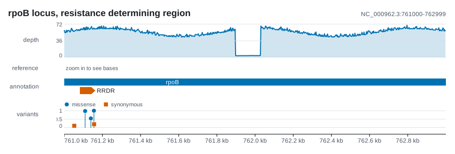
use karyon::{plot, Aggregate, Feature, Strand, Variant};

fn main() -> std::io::Result<()> {
    // Stand-ins for what you would read from files: the depth over
    // 2,000 bases, with a dropout, and the reference bases.
    let depth: Vec<f64> = (0..2_000)
        .map(|i| if (900..1_030).contains(&i) { 3.0 } else { 58.0 })
        .collect();
    let bases: Vec<u8> = b"GCCGGTCA".iter().cycle().take(2_000).copied().collect();

    plot("NC_000962.3:761000-762999")?
        .title("rpoB locus, resistance determining region")
        .add_coverage(depth)
        .label("depth")
        .adjust(|track| track.aggregate(Aggregate::Min).height(70.0))
        .add_sequence(bases)
        .label("reference")
        .add_features(vec![
            Feature::new(759_806, 763_325).name("rpoB").strand(Strand::Forward),
            Feature::new(761_081, 761_162).name("RRDR").strand(Strand::Forward),
        ])
        .label("annotation")
        .add_variants(vec![
            Variant::new(761_108).value(0.98).category("missense"),
            Variant::new(761_154).value(1.00).category("missense"),
            Variant::new(761_155).value(0.21).category("synonymous"),
        ])
        .label("variants")
        .save("rpoB.svg")?;
    Ok(())
}

The figure is what cargo run --example locus draws: the same chain, with depth and bases generated from a seed, the RRDR box coloured, and two more variants.

Three things in that chain happen without being written down:

• The ruler under the tracks was never asked for. The plot adds it.
• The window start is written once, in the locus string. add_coverage and add_sequence start their arrays at the left edge of the region.
• label and adjust act on the track added just above them, not on the figure.

The plot() builder

Start a plot

plot(locus) parses a locus string and returns a Plot over that region.

use karyon::plot;

let figure = plot("chr7:140,753,000-140,754,000")?;

The string is the 1-based, inclusive form that samtools and IGV print. Commas and underscores in the numbers are ignored, and the sequence name may contain colons of its own, because the string is split at the last one. A string that does not parse is an Error::InvalidLocus, never a panic (see Errors).

Only the locus string is 1-based

Every other position in the API is 0-based and half-open, the BED convention, so a VCF POS or a GFF start is pos - 1 on the way in. plot("chr1:101-200") covers the region whose start() is 100 and whose end() is 200, and the ruler prints positions back in the 1-based form. See Coordinates.

Plot::over starts from a Region you already hold, which suits coordinates that are computed rather than typed. region() reads the region back anywhere in the chain.

use karyon::{Plot, Region};

let region = Region::new("NC_000962.3", 761_000, 763_000)?;
let figure = Plot::over(region);

plot_tree() starts a plot of phylogenies, which names no place: a tree's x is a branch length or a time, so it takes no locus, writes none at the top right and draws no ruler.

use karyon::{plot_tree, Tree};

let figure = plot_tree().add_tree(Tree::parse_newick("((A:1,B:1):1,C:2);")?);

One call per track

Each add_ method builds one track and puts it under the tracks already added, so the order of the calls is the order of the stack. There is one for each of the 38 track types the crate ships, five _at forms that take the start of an array, and two that take a track you built yourself.

Method	Adds	Takes
add_axis()	AxisTrack	nothing: the ruler, placed where the call sits
add_bisulfite(sites, molecules)	BisulfiteTrack	Vec<u64>, Vec<Molecule>
add_clades(tree, blocks)	CladeTrack	Tree, Vec<CladeBlock>
add_codons(start, end, strand)	CodonTrack	u64, u64, Strand: the coding sequence
add_copy_number(segments, ploidy)	CopyNumberTrack	Vec<CopyNumberSegment>, f64; the ploidy has no default
add_coverage(values)	CoverageTrack	Vec<f64>, one per base from the left edge of the region
add_coverage_at(start, values)	CoverageTrack	u64, Vec<f64>
add_domains(rows)	DomainTrack	Vec<DomainArchitecture>
add_dotplot(blocks)	DotplotTrack	Vec<AlignmentBlock>
add_dynseq(start, seq, scores)	DynseqTrack	u64, Vec<u8>, Vec<f64> with one score per base
add_features(features)	FeatureTrack	Vec<Feature>
add_genome(genome)	GenomeTrack	Genome
add_genotypes(samples, sites)	GenotypeTrack	Vec<String>, Vec<GenotypeSite> with a call per sample
add_ideogram(length, bands)	IdeogramTrack	u64, Vec<Band>
add_junctions(junctions)	JunctionTrack	Vec<Junction>
add_key()	LegendTrack	nothing: the key every track gives, in the figure's theme, at the foot of the figure
add_legend(legend)	LegendTrack	Legend
add_loci(loci)	LocusTrack	Vec<Locus>
add_logo(columns)	LogoTrack	Vec<LogoColumn>, from the left edge of the region
add_logo_at(start, columns)	LogoTrack	u64, Vec<LogoColumn>
add_manhattan(points)	ManhattanTrack	Vec<Association>
add_matrix(sites, rows)	MatrixTrack	Vec<u64>, Vec<MatrixRow>
add_methylation(sites)	MethylationTrack	Vec<MethylSite>
add_msa(sequences)	MsaTrack	Vec<MsaSequence>
add_orfs(seq)	OrfTrack	Vec<u8>, from the left edge of the region
add_orfs_at(start, seq)	OrfTrack	u64, Vec<u8>
add_phylodynamics(points)	PhylodynamicTrack	Vec<PhylodynamicPoint>
add_pileup(reads)	PileupTrack	Vec<Read>
add_selection(sites)	SelectionTrack	Vec<SelectionSite>
add_sequence(seq)	SequenceTrack	Vec<u8>, from the left edge of the region
add_sequence_at(start, seq)	SequenceTrack	u64, Vec<u8>
add_snps(names, sites)	SnpTrack	any iterator of sample names, Vec<SnpSite>
add_split_reads(reads)	SplitReadTrack	Vec<SplitRead>
add_squiggle(signal)	SquiggleTrack	Vec<f64>, one per sample from the left edge of the region
add_squiggle_at(start, signal)	SquiggleTrack	usize, Vec<f64>
add_structural(variants)	StructuralTrack	Vec<StructuralVariant>
add_surveillance(observations)	SurveillanceTrack	Vec<SurveillanceObservation>
add_synteny(blocks)	SyntenyTrack	Vec<AlignmentBlock>
add_tanglegram(left, right)	TanglegramTrack	Tree, Tree
add_transcription_units(units)	TranscriptionUnitTrack	Vec<TranscriptionUnit>
add_tree(tree)	TreeTrack	Tree
add_variants(variants)	VariantTrack	Vec<Variant>
add_windows(windows)	WindowTrack	Vec<Window>
add_track(track)	any track, already built	impl Track + 'static; leaves nothing pending
add_boxed(track)	any track, already built	Box<dyn Track>; leaves nothing pending

Every Vec<T> in the table is really impl Into<Vec<T>>, so a Vec or an array goes in as it is. Tracks has what each track draws and every option its builder takes.

A track you built yourself

add_track takes a track that is already built. That covers a track from an alternative constructor, a track you need to read before it is drawn, and a track type from outside the crate.

Alternative constructors compute a track from raw input, and there are too many to give each an add_ of its own: WindowTrack::gc_skew, WindowTrack::ratios, SnpTrack::from_alignment, LogoTrack::from_sequences and IdeogramTrack::bare among them.

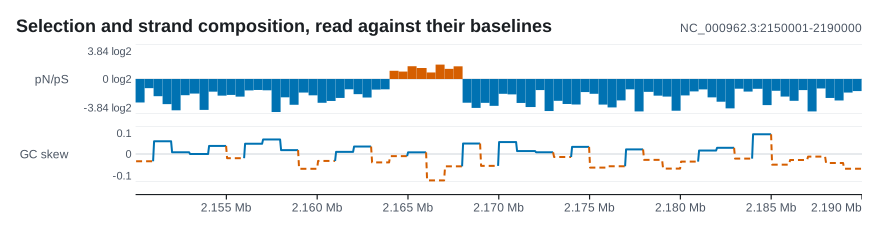
use karyon::{Plot, Region, WindowStyle, WindowTrack};

Plot::over(Region::new("NC_000962.3", start, start + 40_000)?)
    .title("Selection and strand composition, read against their baselines")
    .add_track(WindowTrack::ratios(windows).label("pN/pS").height(70.0))
    .add_track(
        WindowTrack::gc_skew(start, &bases, 1_000)
            .style(WindowStyle::Line)
            .label("GC skew"),
    )

Name the track before you hand it over. add_track leaves nothing pending, so the plot's label and adjust cannot reach it; the track's own label builder is the method Plot::label calls anyway.

Some tracks answer questions about their own data, and the rest of the figure is often placed by the answer: CodonTrack::span_of gives the reference span of a codon, SnpTrack::sites lists the variable sites a panel kept, and TanglegramTrack::crossings counts the crossing ties. Reading one needs the track as a variable, so build it first and add it with add_track:

use karyon::{CodonTrack, Plot, Region, Strand, Variant};

let ruler = CodonTrack::new(759_806, 763_325, Strand::Forward)
    .sequence(view_from, bases)
    .label("rpoB");
let s450 = ruler.span_of(450).expect("rpoB has a codon 450");

Plot::over(Region::new("NC_000962.3", view_from, view_to)?)
    .add_variants(vec![Variant::new(s450.0 + 1).category("S450L")])
    .label("variants")
    .add_track(ruler)

The variant lands on the codon the ruler numbers 450 because both come from one object, not from the same arithmetic done twice.

add_boxed does the same for a Box<dyn Track>, which is what a stack chosen at run time ends up holding. Both take any implementation of the Track trait, your own included: see Writing a track.

A ruler passed to add_track is a second ruler

add_track cannot tell an AxisTrack from any other track, so add_track(AxisTrack::new()) adds a ruler on top of the automatic one. add_axis() is the call that moves the ruler.

Label and adjust

label names the track the last add_ built, in the gutter on the left. adjust hands that track to a closure, for everything else its builder can set.

use karyon::{plot, Aggregate, CoverageStyle};

plot("chr7:140,753,000-140,754,000")?
    .add_coverage(depth)
    .label("depth")
    .adjust(|track| {
        track
            .aggregate(Aggregate::Min)
            .style(CoverageStyle::Area)
            .height(70.0)
    })

The closure receives the track's own type, here a CoverageTrack, so every builder method of that type is in reach. A method the track does not have is a compile error, not a setting ignored when the figure is drawn:

plot("chr7:140,753,000-140,754,000")?
    .add_coverage(depth)
    .add_features(genes)
    .adjust(|track| track.aggregate(Aggregate::Min))

error[E0599]: no method named `aggregate` found for struct `FeatureTrack` in the current scope
  |
  |         .adjust(|track| track.aggregate(Aggregate::Min))
  |                               ^^^^^^^^^ method not found in `FeatureTrack`

The track a plot remembers

A plot holds the track the last add_ built instead of handing it to the figure at once, and it holds it in its type: add_coverage returns a Plot<CoverageTrack>, add_features a Plot<FeatureTrack>, and so on down the chain. That is how adjust gets the concrete type without any downcasting.

A fresh plot is a Plot<Empty>. Empty is not a track, so label and adjust do not exist until something has been added:

error[E0599]: the method `label` exists for struct `Plot`, but its trait bounds were not satisfied
  |
  = note: the following trait bounds were not satisfied:
          `karyon::plot::Empty: karyon::plot::Named`

Which track a call reaches is not checked

It is decided by where the call sits. An adjust written one add_ too late configures the next track, and compiles whenever that track has the same method:

plot("chr7:140,753,000-140,754,000")?
    .add_coverage(depth)
    .label("depth")
    .add_sequence(bases)
    .adjust(|track| track.height(70.0)) // the sequence, not the depth

Every track has label, so a misplaced label always compiles and always names the wrong row. Read a chain by its add_ calls, and treat what follows each one as belonging to it.

The pending track goes into the figure when the plot moves on:

Call	The pending track	Returns
the next add_	is added to the figure	a plot holding the new track
add_track, add_boxed	is added, then the track you pass	Plot<Empty>
done()	is added	Plot<Empty>
save(path)	is added, and the ruler appended	Plot<Empty>
into_figure(), to_svg(), to_pdf()	is added, and the ruler appended	the Figure, the SVG, or the PDF

A stack built in a loop. Every arm of a loop or an if must have one type, and a plot's type changes with every add_. done() puts the pending track away and returns a Plot<Empty>, a type that stays the same:

let mut figure = plot("chr2:1-4,000")?;
for (name, depth) in samples {
    figure = figure.add_coverage(depth).label(name).done();
}
figure.save("samples.svg")?;

done draws nothing and decides nothing. It is the point where the plot stops naming the track it holds.

A plot passed to a function. Plot on its own means Plot<Empty> and will not accept a plot in the middle of a chain. Make the function generic over T: Slot (from karyon::plot), or pass it the Figure that into_figure returns. Slot is sealed: a track type from outside the crate goes in through add_track, not by implementing it.

What a plot fills in

Two things happen without being asked, and both can be undone.

The ruler under the tracks

A figure with no coordinates along it is rarely what anyone meant, so the plot adds an AxisTrack when it becomes a figure, under the last track laid on the coordinates. A tree or a panel of sites below that track stays below the ruler, which numbers what is above it and not them. The plot leaves the ruler out when nothing in the stack is laid on the coordinates: a plot of nothing but phylogenies (add_tree, add_tanglegram) gets none, because a tree's x is a branch length, not a position in the region.

• add_axis() puts the ruler where the call sits, above a track or between two, and the automatic one is then not added, so there is still exactly one.
• remove_axis() leaves the automatic ruler out. It can sit anywhere in the chain, since it is a decision about the finished figure, and it leaves a ruler placed with add_axis or add_track where it is.

plot("chr1:1-1000")?
    .add_axis()
    .add_coverage(depth)
    .label("depth")

The ruler counts whatever the region counts, and a region is a coordinate system, not a claim about a genome. An alignment is indexed by column and a raw signal by sample, so a plot of one wants a region in that unit, such as plot("alignment:1-320"), and the ruler then counts columns. plot_alignment(rows) is that plot of an alignment without the arithmetic: as many columns as its longest row, no locus printed, the alignment drawn, and a ruler that counts columns.

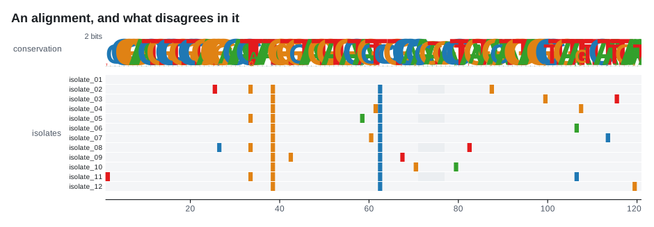
The locus printed at the top right is then the one thing that still reads as genomic, so remove_region_label() leaves it out:

plot(&format!("alignment:1-{columns}"))?
    .title("An alignment, and what disagrees in it")
    .remove_region_label()

The start of an array

A coverage profile, a reference sequence, a set of reading frames, a logo and a raw signal are arrays laid along the axis, and each needs to know where its first element sits. Almost always that is the left edge of the region, which the plot already holds:

plot("NC_000962.3:761001-762000")?
    .add_coverage(depth) // depth[0] is at 0-based 761,000

When the array starts somewhere else, the _at form takes the start. A profile over the second half of the window:

plot("NC_000962.3:761001-762000")?
    .add_coverage_at(761_500, depth)

add_coverage(values) is exactly add_coverage_at(region.start(), values). A squiggle counts samples rather than bases, so add_squiggle_at takes a usize and add_squiggle converts the region start to one. add_dynseq has no implicit form: it always takes its start.

Figure settings

These set the figure, not a track. They leave the pending track alone, so they can sit anywhere in the chain.

Method	Default	Sets
width(f64)	900.0	the image width in pixels
title(impl Into<String>)	none	the bold line above the tracks
theme(Theme)	Theme::light()	colours and fonts: see Styling
profile(RenderProfile)	the Manuscript values	theme, visual scale and density in one call
visual_scale(f64)	1.0	type, marks, bands, margins, gaps and corners together; never the coordinates, and the width only where it is below the floor
density(Density)	Density::Balanced	how tightly repeated rows and marks are packed
margin(Margin)	14, 18, 14, 16	whitespace top, right, bottom and left
label_width(f64)	measured	the width of the left gutter that holds track labels
track_gap(f64)	12.0	the vertical gap between tracks
remove_region_label()	shown	leaves out the locus at the top right
remove_axis()	appended	leaves out the automatic ruler
same_scale()	each track to its own values	draws the tracks that measure the same thing on one scale: several depths read off one ceiling (--same-scale)
shade(Shade)	none	shades a stretch down every band laid on the coordinates, as .shade(Shade::new(1_450_000, 1_510_000).name("deletion")); once for each stretch (--shade)

• The height is not a setting. It follows from the tracks, each of which says how tall it wants to be. See How the layout works.
• same_scale shares a scale between tracks that measure one thing: coverage in the same units on the same kind of scale, windows about the same baseline, scans of the same statistic. A track whose maximum you pinned keeps it. Across the panels of a sheet, join what each figure measures with Extent::join over Figure::extents, and hand the result to each one's Figure::share_extents; the command line does this for a figure of several places.
• shade marks a stretch down the whole stack, 0-based and half-open as every track's coordinates are. The wash goes behind the tracks, so no colour in them changes, and its two ends are dashed lines drawn over them, so a heatmap whose cells hide the wash still shows where the stretch is. It is drawn only across bands on the coordinates: a tree, an ideogram or the key breaks the column and it goes on under them, and synteny is left out because its lower bar is the other sequence. A name, Shade::name, is written at the head of the column, and the alt text says every stretch in view. One colour for every shade is the default, since a shade says look here and not which category; Shade::color gives one its own.
• profile replaces the theme, the visual scale and the density, so call it before any of the three you want to set yourself. The profiles are on Styling.
• The label gutter is only reserved when at least one track has a label. Its width follows the widest label, between 48 and 160 pixels, and label_width fixes it for a layout that must not move.
• The alt text is set with description, which is on Figure and not on Plot: into_figure().description("...").

Render and save

to_svg() returns the figure as a standalone SVG document in a String, and to_pdf() the same drawing as a PDF. save(path) writes it, as PDF when the name ends in .pdf and as SVG under any other, and hands the plot back, which lets one stack be drawn twice:

use karyon::{plot, Theme};

plot("plasmid:1-2000")?
    .add_coverage(depth)
    .save("light.svg")?
    .theme(Theme::dark())
    .save("dark.pdf")?;

A save closes the stack: it puts the pending track away and appends the ruler. Saving twice therefore does not draw two rulers, and a track added after a save sits below the ruler rather than above it.

into_figure() hands over the Figure, with the pending track and the ruler in place. It is the way out to anything that wants a figure: dimensions(), description(), to_svg_with_id_prefix(), or a Panels sheet.

use karyon::{plot, Panels};

let top = plot("chr1:1-1000")?.add_coverage(depth).into_figure();
let bottom = plot("chr1:1-1000")?.add_manhattan(points).into_figure();

Panels::new().push(&top, "A").push(&bottom, "B").save_svg("sheet.svg")?;

Errors

Failure sits at the two ends of a program that draws: reading a locus, a tree or a file's text at the start, and writing the SVG at the end. Nothing in between returns a Result, and rendering never fails.

Call	Fails with
plot(locus), Region::parse(locus)	Error::InvalidLocus: no colon, no dash after it, an empty name, a coordinate that is not a whole number, a start of 0, or an end before the start
Region::new(seq, start, end)	Error::EmptyRegion when end <= start
Genome::checked(sequences)	Error::DuplicateSequence when two sequences share a name
Tree::parse, Tree::parse_all, Tree::parse_newick, Tree::parse_annotated_newick, Tree::parse_nexus	Error::InvalidNewick, Error::InvalidNexus
the readers in karyon::read	ReadError, with the line number and the reason: see File formats
save, save_svg, save_pdf, Pdf::save	the std::io::Error of the write

karyon::Error converts into std::io::Error, so a function that returns std::io::Result can use ? on the locus and on the file alike, as the program at the top does. ReadError has no such conversion: map it, or return Box<dyn std::error::Error>.

Data that cannot be drawn as asked is drawn as well as it can be, not refused: a coverage array that runs out before the region does stops where it stops, a feature that begins before the window keeps its real start and is clipped, and a width too small to leave a plotting area is raised to the smallest one that does.

Figure: full control

Figure is what plot() builds. Use it directly when the tracks are values you build, store, pass around or return. Neither layer draws anything the other cannot: the same stack written both ways renders the same document, byte for byte, and a test in src/plot.rs holds them to it.

With plot()With Figure

plot("NC_000962.3:761001-762000")?
    .title("a locus")
    .add_coverage(depth)
    .label("depth")
    .add_features(genes)
    .label("genes")
    .to_svg()

Figure::new(Region::parse("NC_000962.3:761001-762000")?)
    .title("a locus")
    .push(CoverageTrack::new(761_000, depth).label("depth"))
    .push(FeatureTrack::new(genes).label("genes"))
    .push(AxisTrack::new())
    .to_svg()

Build a stack

use karyon::{AxisTrack, CoverageTrack, Figure, Region};

fn main() -> std::io::Result<()> {
    let depth: Vec<f64> = (0..2_000).map(|i| 30.0 + (i % 40) as f64).collect();

    Figure::new(Region::parse("chr7:5,220,001-5,222,000")?)
        .title("A locus")
        .push(CoverageTrack::new(5_220_000, depth).label("depth"))
        .push(AxisTrack::new())
        .save_svg("locus.svg")?;
    Ok(())
}

Region::parse turns the 1-based chr7:5,220,001-5,222,000 into the 0-based, half-open span [5220000, 5222000), which is why the coverage starts at 5_220_000. A Figure adds nothing on its own, so the ruler is pushed explicitly.

push appends a track below the ones already there, so the order of the push calls is the order of the stack. Nothing about a track depends on where it sits, so reordering a figure is reordering its calls.

push_boxed takes a Box<dyn Track>, which is what a stack built in a loop or behind a condition needs: each arm produces a different track type, and a boxed trait object is the one thing they have in common.

use karyon::{AxisTrack, CoverageTrack, Figure, Region, Track};

let mut tracks: Vec<Box<dyn Track>> = Vec::new();
for (name, depth) in samples {
    tracks.push(Box::new(CoverageTrack::new(0, depth).label(name)));
}
tracks.push(Box::new(AxisTrack::new()));

let mut figure = Figure::new(Region::new("chr2", 0, 4_000)?);
for track in tracks {
    figure = figure.push_boxed(track);
}

How the layout works

A track knows two things: how tall it wants to be and how to draw itself. It is never told where it sits. The figure decides the rest.

+--------------------------------------------------------------------+
|  A locus                                     chr7:5220001-5222000  |  header
|                                                                    |
|       depth |  40 |    ____        ___                             |  band 0
|             |   0 |___/    \______/   \____                        |
|  - - - - - - - - - - - - - - - - - - - - - - - - - - - - - - - -   |  track_gap
|       genes |     |   >>>>>>>>>>       <<<<<<<                     |  band 1
|                                                                    |  track_gap
|             |     |  |      |      |      |                        |  band 2
+--------------------------------------------------------------------+
    \________/ \___/ \_____________________________________________/
      label    value              plotting area
      gutter   axis

The box is the image, and the space between it and the content is the margin. The figure settles the pieces in this order:

1. The header, present when there is a title or a region label, and title_font_size + 12 pixels tall. The title is drawn bold at the left and shortened with an ellipsis if it would run into the locus, which is drawn in the muted colour at the right.
2. The label gutter, reserved only when at least one track has a label. Its width follows the widest label plus 14 pixels, kept between 48 and 160, unless label_width sets it. Labels are set semibold in the muted ink, in the case they were given, right-aligned against the value axis, and a label wider than the gutter is shortened with an ellipsis.
3. The value axis strip. Each track says how much room it wants for its own ticks. The figure gives every track the widest of those requests, so all plotting areas start at the same x. A coverage track asks for room to print its values; a pileup or a sequence asks for none.
4. The bands. Each track gets a band as wide as the plotting area and as tall as it asked, stacked in push order with track_gap between them. Each is clipped to its band and the axis strip it asked for, so a track cannot paint into its neighbour: a feature that starts before the window is drawn whole and the clip cuts it. A hairline separates two labelled tracks that follow each other, when the gap between them is at least 6 pixels.
5. The row of shade names, one line of type plus 8 pixels, 19.5 at the plain scale, directly above the first band that shows shades, and only while a named shade is in view. A shade outside the window takes no room at all, and an unnamed one none either.
6. The height, computed rather than configured: margin.top + header + sum of the track heights + track_gap * (n - 1) + name row + margin.bottom. That is why dimensions() has to lay the figure out to answer.

A shade is the one mark the figure draws across bands, since no track can reach outside its own. Its wash is drawn before any track, down each run of bands in a row whose track shows shades, across the gaps between them, from the plotting area's left edge at most, so never into the gutter or an axis strip. Its edges are drawn after every track. A shade under 2 pixels wide is widened to 2, and one under 6 has a single edge down its middle.

Every length in that list is multiplied by the visual scale, and the track heights by the density as well. A track's height comes from Track::height(&scale), and the scale is passed in because some tracks change height with zoom: a feature track needs more rows when features overlap on screen, so the same track is shorter zoomed in than zoomed out.

Tracks that do not map through the shared scale

Most tracks place their data through one shared Scale, which is what keeps the x axes aligned. A few draw against their band instead, because their x is not a position in the region: IdeogramTrack draws the whole chromosome and marks the region on it, SnpTrack spaces its variable sites evenly, TreeTrack and TanglegramTrack draw branch lengths, and LegendTrack is a key.

Size and spacing

Figure takes the settings in the plot's table, with two differences: show_region_label(false) stands in for remove_region_label(), and there is no remove_axis(), since a figure holds only the tracks you push. It adds description(text) for the alt text. Each setting is a consuming builder method, so they chain in any order, profile aside.

use karyon::{Figure, Margin, Region, Theme};

let figure = Figure::new(Region::new("contig_01", 0, 50_000)?)
    .width(1_200.0)
    .theme(Theme::dark())
    .visual_scale(1.15)
    .margin(Margin { top: 14.0, right: 20.0, bottom: 14.0, left: 16.0 })
    .label_width(120.0)
    .track_gap(6.0)
    .show_region_label(false);

Margin has four public f64 fields, top, right, bottom and left, and its Default is 14, 18, 14, 16. top is the space above the title and left the space to the left of the track labels.

Values that would break the document are corrected rather than passed through. A width too small to leave a plotting area is raised to the smallest one that does, and a width that is not a finite number is replaced by that floor. The floor depends on the margins, label_width and the visual scale, so it is worked out when the figure is laid out: width written before them draws the same figure as width written after, and the default of 900 is held to it too. A margin side or a label_width that is negative or not finite becomes zero, and so does a negative track_gap. A visual_scale below 0.25 is raised to it, and one that is not finite is taken as 1.0.

Read a figure back

let (width, height) = figure.dimensions();
println!("{width} x {height}, {} tracks", figure.track_count());
println!("{}", figure.region());

dimensions() is the one that does work: the height follows from the tracks, so asking for it means laying the figure out. region() prints in the 1-based inclusive form, the same string as the region label. measures_coordinates() says whether a ruler would measure anything, which is what plot() asks before appending one, and shades() gives back the stretches shaded, in the order they were given.

Render a figure

to_svg() returns a standalone SVG 1.1 document as a String, and save_svg(path) renders and writes it, returning whatever the write returns. to_pdf() and save_pdf(path) do the same as PDF. The save, save_svg and save_pdf methods, and Pdf::save, are the only calls in the library that write a file.

Every document names and describes itself for screen readers. Its <title> is the title and the locus, or the locus alone, and its <desc> defaults to a list of what the figure holds: the region, the number of tracks, and each track top to bottom, by its label or, where it has none, by what it is, a ruler or a phylogeny. Only you know what the figure shows, so say it with description:

use karyon::{AxisTrack, Figure, Region};

let svg = Figure::new(Region::parse("chr7:1-1000")?)
    .description("Read depth falls to zero across the deleted exon.")
    .push(AxisTrack::new())
    .to_svg();

to_svg_with_id_prefix(prefix) renders the same drawing with every id it generates starting with prefix, for nesting it inside another SVG by hand. Panels does this for you.

Why nested figures need their own ids

Ids in SVG belong to the whole document, and url(#id) resolves to the first match anywhere in it. Two figures nested in one document would both claim karyon-clip-0, and the second one's tracks would be clipped to the first one's bands. A prefixed render also leaves out its own <title> and <desc>, since a nested drawing must not name itself: the document it goes into does that.

PDF

to_pdf() returns a Pdf: its bytes, from %PDF to %%EOF, and its notes, each way the page differs from the SVG it was converted from, for a person to read. The notes are empty for everything the crate draws unless a label holds a character no base font has, such as a sample name in Cyrillic, which is drawn as a question mark and named.

use karyon::{plot, Pdf};

let figure = plot("chr1:1-1000")?.add_coverage(depth).into_figure();
let pdf = figure.to_pdf();
assert!(pdf.notes.is_empty());
pdf.save("depth.pdf")?;

// Any SVG written in the same terms converts, such as a drawing of your own.
let pdf = Pdf::from_svg(&figure.to_svg()).expect("a root <svg> with a size");

The PDF is read from the SVG rather than drawn a second time, its text is set in Helvetica, Courier and Symbol with no font embedded, and a pixel is three quarters of a point. How the PDF is made says what that keeps and what it changes.

Panels: several drawings on one sheet

A figure in a paper is usually several plots with letters on them. Panels puts finished drawings on one SVG sheet, each with an optional letter and caption, without any of them knowing about the others.

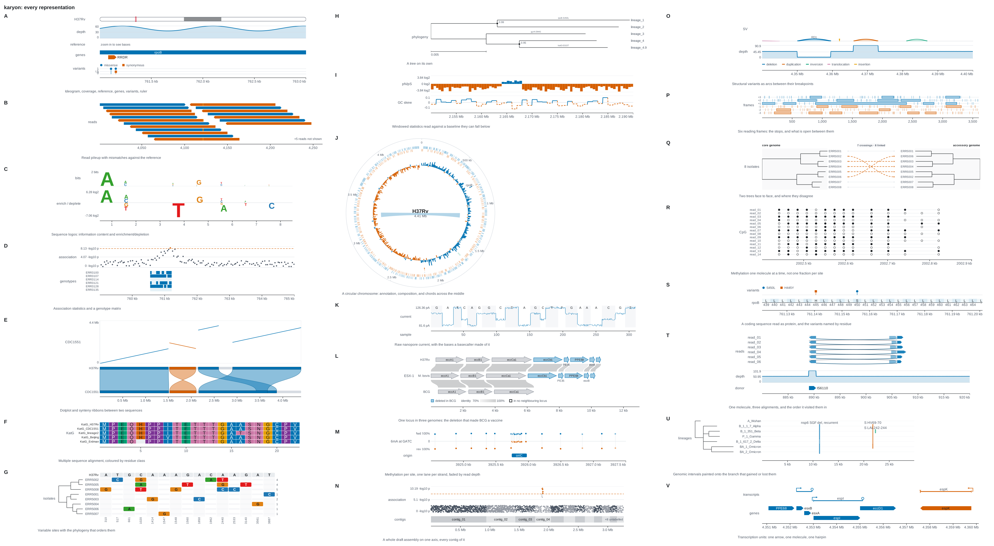
use karyon::Panels;

let sheet = Panels::new()
    .title("Figure 1")
    .columns(2)
    .gap(20.0)
    .push_captioned(&stack, "A", "Read depth and annotation across the locus")
    .push_captioned(&circle, "B", "The same sample as a closed sequence");

sheet.save_svg("figure-1.svg")?;

Add a drawing with push(&drawing, letter), push_captioned(&drawing, letter, caption) or push_bare(&drawing). Each renders the drawing when it is added and keeps the result, so a later change to the drawing does not reach the sheet.

Method	Default	What it does
columns(usize)	1	lays the panels out in this many columns
row_major()	column by column	fills each row left to right before starting the next
gap(f64)	18.0	the vertical gap between panels
column_gap(f64)	26.0	the horizontal gap between columns
margin(f64)	14.0	whitespace around the sheet
title(impl Into<String>)	none	a bold line across the top
description(impl Into<String>)	the letters and captions	the sheet's alt text
theme(Theme)	Theme::light()	the sheet's own page, title, letters and captions; each panel keeps its own theme
profile(RenderProfile)	the Manuscript values	the sheet's theme and visual scale
visual_scale(f64)	1.0	scales the panels, letters, captions, gaps and margins together, panels already added included
align_plot_areas(bool)	true	starts the data of every linear figure at the same x

len(), is_empty() and dimensions() read the sheet back; to_svg(), save_svg(path), to_pdf() and save_pdf(path) render it, the PDF as one page with each panel clipped to its own box.

• Column by column. Panels fill each column top to bottom before starting the next, so the letters still read in order, as they do down the columns of a paper. Where each column ends is chosen by weighing every possible cut: the tallest column is made as short as it can be, then the others are levelled.
• Row by row. row_major() makes a grid instead: A and B share the first row, C and D the second, and each row is as tall as its tallest panel. Use it when the rows mean something, as in a comparison.
• Aligned data. A panel with a long track label and a panel with no gutter still start their data at the same x. Circular plots and other drawings with no linear origin keep their own left edge. align_plot_areas(false) releases the alignment for a grid that mixes unrelated coordinate systems, such as a rectangular tree, a radial tree and an alignment.
• Letters and captions. Letters get a strip of their own left of each column, since a letter drawn over a panel is drawn over data, and over an opaque page it is not seen at all. A caption sits under its panel in the muted colour, and a caption wider than its panel widens the column rather than running into the next one.

How a panel goes onto the sheet

Each panel is nested whole, as an <svg> inside a group that moves it, so a panel on a sheet is the same picture as the panel on its own. Nothing is parsed again or rewritten. Its ids are the one thing it cannot keep to itself, so each panel is rendered with a prefix of its own and its clips go on pointing at its own bands. The sheet names itself in its <title> (its title, or how many panels it holds), its <desc> lists the letters and captions unless description says otherwise, and hovering a panel shows its letter and caption.

What can go on a sheet

A sheet takes anything that implements Drawing, which asks for a size and a rendering:

pub trait Drawing {
    fn dimensions(&self) -> (f64, f64);
    fn to_svg_with_id_prefix(&self, prefix: &str) -> String;
    fn content_anchor(&self) -> Option<f64> {
        None
    }
}

Figure, Rings, Map and PhyloMap implement it, so a stack and a circle share a sheet without having anything else in common: panel J of the sheet above is a Rings plot. content_anchor is where the data starts, for align_plot_areas; a Figure returns the left edge of its plotting area and the others keep the default. A function can take any of them:

use karyon::{Drawing, Panels};

fn sheet(a: &impl Drawing, b: &impl Drawing) -> Panels {
    Panels::new().push(a, "A").push(b, "B")
}

Rings: a circular sequence

A plasmid, an organelle genome, many viral genomes and most bacterial chromosomes have no ends. Drawn as a line, the sequence gets an edge the biology does not have, straight through whatever sits at coordinate zero. Rings maps position to an angle instead, which is a different coordinate system and so a different container: Rings is to Ring what Figure is to Track. From the command line, --circular draws the place, one whole sequence, this way, a ring for each track; A whole sequence shows it.

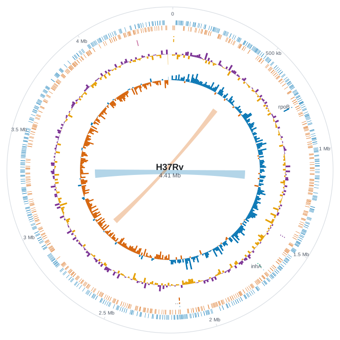
use karyon::{AxisRing, FeatureRing, MarkerRing, Rings, SignalRing};

Rings::new(4_411_532)
    .diameter(660.0)
    .title("H37Rv")
    .subtitle("4.41 Mb")
    .push(AxisRing::new())
    .push(FeatureRing::new(genes).thickness(20.0))
    .push(MarkerRing::categorised(mutations).thickness(12.0))
    .push(SignalRing::new(gc_content).thickness(44.0))
    .push(SignalRing::new(gc_skew).thickness(50.0))
    .link((1_100_000, 1_180_000), (3_240_000, 3_320_000))
    .save_svg("H37Rv.svg")?;

The figure is cargo run --example circular, which also draws a thin ring naming three loci, reads GC content against the GC content of the whole sequence, sets colours of its own and adds a second chord.

Position zero is at twelve o'clock and coordinates run clockwise, the convention of circular genome viewers. The first push takes the outermost radius and each ring after it sits inside the last, so push the ring with the most detail first: an arc on an outer ring has more pixels than the same arc further in.

Ring	Draws	Builder methods, with defaults
AxisRing::new()	a ruler of positions	thickness (22), ticks (10), show_labels (true)
FeatureRing::new(features)	annotation as arcs, forward strand outside and reverse inside, each feature in its own color where it has one	thickness (16), colors(forward, reverse), split_strands (true), show_names (false), min_degrees (0.12)
SignalRing::new(windows), SignalRing::from_spans(length, spans, bins, aggregate)	a quantity in windows, either side of a baseline circle; from_spans cuts a per-base signal, as a depth file states it, into bins equal arcs, each the Aggregate of the bases under it	thickness (40), baseline (0), baseline_at_median(), colors(above, below), extent, show_baseline (true)
MarkerRing::new(positions), MarkerRing::categorised(pairs)	points as radial ticks; categorised takes (position, category) pairs and gives each category a palette colour	thickness (10), width (1.2), colors to replace the palette

Every ring takes label, its name. A ring has nowhere to write one, so a named ring is one tooltip, its name, wherever a pointer lands on it and no mark of its own answers first, and key(name, legend) on Rings writes it out under the circle: a line a ring, its name and then what its colours mean, in the order added. Add them in the order the rings were pushed and the key reads outside in, as the circle does.

What a circle adds over a stack of bands is the middle. link(from, to) draws a translucent ribbon between two spans that belong together: the two ends of an inversion, a duplication and its source. Both spans are (start, end), 0-based and half-open, and a span whose end is below its start runs through the origin. link uses the theme's accent at an opacity of 0.35, and link_colored(from, to, color, opacity) takes an Option<String> colour and an opacity of its own. Chords are drawn before the rings, so a dozen of them crossing the middle do not wash the data out. An end narrower than 0.3 degrees, a breakend's single base above all, is drawn that wide, centred on its span, and its tooltip still says the base.

Method	Default	What it does
diameter(f64)	640.0	the diameter of the outermost ring, at least 80 pixels
margin(f64)	14.0	whitespace around the circle
origin_gap(f64)	2.0	degrees left blank at twelve o'clock, from 0 to 90
title(impl Into<String>)	none	the name written in the middle
subtitle(impl Into<String>)	none	a second, quieter line under it
description(impl Into<String>)	the length, the rings and the chords, counted, and the rings' names, outside in	the alt text
key(name, Legend)	none	a line of the key under the circle; the image grows downwards to hold it
theme(Theme)	Theme::light()	colours and fonts
profile(RenderProfile)	the Manuscript values	theme, visual scale and ring density together
visual_scale(f64)	1.0	type, marks, margins and ring thickness together
density(Density)	Density::Balanced	how tightly the rings are packed

The two-degree gap at the origin is there on purpose: a closed circle hides the fact that a coordinate system has to start somewhere, and that the choice was arbitrary. origin_gap(0.0) closes it.

length(), ring_count(), dimensions() and inner_radius() read the plot back, the last being the radius where chords start. push_boxed, to_svg, to_svg_with_id_prefix, save_svg, to_pdf and save_pdf work as they do on Figure. A ring type of your own implements the Ring trait: thickness(), an optional gap() (5 pixels by default), an optional label() (none by default) and draw(ctx), which draws between the two radii in the RingContext it is given.

Genome: several sequences on one axis

A figure is one region on one sequence, which is right for a locus and wrong for an assembly: two hundred contigs, a couple of dozen chromosomes, or a chromosome and its plasmid. Genome lays the sequences end to end and hands back one region that covers them all, and every track then works across all of them at once.

use karyon::{Figure, Genome, GenomeTrack};

let genome = Genome::new([
    ("chrI", 230_218u64),
    ("chrII", 813_184),
    ("chrIII", 316_620),
]);

assert_eq!(genome.total(), 1_360_022);

// A position on one sequence becomes a position on the shared axis.
let at = genome.at("chrII", 1_000).unwrap();
assert_eq!(at, 231_218);
assert_eq!(genome.locate(at), Some(("chrII", 1_000)));

Figure::new(genome.region())
    .push(GenomeTrack::new(genome.clone()).label("chromosomes"))
    .save_svg("genome.svg")?;

The order you give is the drawing order and is never sorted: a reference is conventionally ordered by chromosome number and an assembly by contig length, and neither is something to guess.

Method	Returns
total()	the length of the whole axis, gaps included
region()	the region covering every sequence, named genome
sequences()	the Chromosome list, each with a name and a length
len(), is_empty()	how many sequences there are
offset(name)	where a sequence starts on the shared axis, or None
at(name, pos)	a position on one sequence as a position on the shared axis, or None
locate(pos)	the inverse: the sequence and offset a shared position falls on, or None
boundaries()	where each sequence starts, for ManhattanTrack::bands
spans()	each sequence as its name and the two ends of its span
map(items)	(name, pos, value) triples placed on the axis, and how many were dropped

at returns None when the genome has no sequence of that name, which is what a naming mismatch between a variant file and a reference looks like (chr1 against 1), and when the position is past the end of its sequence, which is what a different reference build or unconverted 1-based positions look like. Nothing normalises a name. map does the same for a whole list and reports how many it dropped, so you can say how many went missing rather than wonder why the figure looks thin:

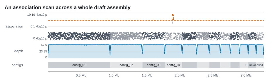
use karyon::{Association, Plot};

let (mapped, dropped) = genome.map(hits);
if dropped > 0 {
    eprintln!("{dropped} points did not land on a sequence of this genome");
}
let points: Vec<Association> = mapped
    .into_iter()
    .map(|(at, value)| Association::new(at, value))
    .collect();

Plot::over(genome.region())
    .title("An association scan across a whole draft assembly")
    .remove_region_label()
    .add_manhattan(points)
    .label("association")
    .adjust(|track| track.bands(genome.boundaries()))
    .add_genome(genome.clone())
    .label("contigs")

Genome::checked refuses a repeated name with Error::DuplicateSequence, since at would otherwise place everything on the first of the two. gap(bases) puts blank axis between one sequence and the next, which shows the joins without any drawing at the cost of coordinates that belong to no sequence: locate returns None inside a gap.

A concatenated axis is not a ruler

A distance measured across a boundary is not a distance. Two points a pixel apart may be the last base of one contig and the first of the next, which are not neighbours in any sense that matters. GenomeTrack draws where the joins are and names each sequence rather than printing coordinates of a concatenation nothing else uses. The ruler a plot appends still counts the concatenated axis; remove_axis() leaves it out.

Where next

• Tracks

  What each add_ builds, every option its builder takes, and what it refuses to draw.

• Styling

  The two themes, every colour and size a figure shares, and the named profiles.

• Command line

  The same stack written as flags, one track per flag, in stack order.

• Writing a track

  The Track trait: what a figure asks of a track and what it does on the track's behalf.