Recipes
Short, complete answers to common tasks, grouped by what you are trying to do. Each one runs as written once its input files exist.
Two conventions run through all of them. A locus string is 1-based and
inclusive, the way samtools and IGV write it, while positions inside the API
are 0-based and half-open, so chr1:101-200 starts at 100 and ends at 200. And
tracks stack in the order they are written, as add_ calls or as flags.
In the Rust fragments, depth is a Vec<f64> holding one value per base of
the region, genes a Vec<Feature> and variants a Vec<Variant>; any
other input is described beside its code.
-
Depth from a BAM, a bedGraph beside a BED, a signed statistic in windows, and a cohort landscape.
-
The files a pipeline wrote, the same stack at base resolution, and the reads under a call.
-
A track per sample, only the sites that vary, and a tree beside them.
-
A scan with the genotypes under it, and a scan across a whole assembly.
-
Support, branch events and distance on one tree, and two trees face to face.
-
Dark and wide, light and dark from one stack, a sheet of panels, and a figure inside a page.
Coverage and signal
Depth over one gene, straight from a BAM
Plot read depth across one gene, with the gene found in the annotation.
katG is looked up in genes.gff3, and the figure is the gene with a tenth of
its length either side, titled with its name. aln.bam is drawn as its depth,
counted the way samtools depth -a counts it, and read through aln.bam.bai
when it is there, so only the reads over the gene are read. Put --pileup in
front of the BAM to draw the reads themselves.
One track per command can read standard input
Any track file can be -, but only one track can take it, since there is
only one standard input to go round.
A bedGraph beside a BED
The shortest real figure: a value per base and a few intervals, from the two commonest text files in a genomics directory.
karyon chr7:140,753,001-140,754,000 \
  --coverage depth.bedgraph --label depth --aggregate min \
  --features genes.bed      --label genes \
  -o locus.svg
Both files are 0-based and half-open, the crate's own convention, so they pass straight through. Only the region is 1-based, because that is what you copy out of a genome browser. A BED with no strand column draws plain blocks without arrowheads, and column 4, when there is one, names each block.
A signed statistic in windows
Draw a statistic that crosses zero, such as GC skew, on both sides of its line, above a read depth on a log scale.
karyon contig_01:1-900,000 \
  --windows gc-skew.bedgraph --label 'GC skew' --style steps \
  --coverage depth.bedgraph  --label depth --log \
  -o skew.svg
A window track draws against a baseline rather than up from the floor of its
band, and colours each window by the side it fell on. GC skew and Tajima's D
change sign, and a statistic like that drawn up from zero loses the one thing
it was computed to say. A read depth cannot go below zero, which is why
--coverage is a separate track rather than a style; --log keeps a
collapsed repeat from flattening the rest of it. The command line draws the
line at zero. In the library, WindowTrack::ratios draws a ratio such as
pN/pS as log2 around one, and baseline moves the line anywhere else.
--style takes steps or line for a window track, area, line or bars
for coverage, tick or lollipop for variants, and differences or all for
an alignment. A word the track does not take is an error that lists the ones
it does.
A cohort copy number landscape
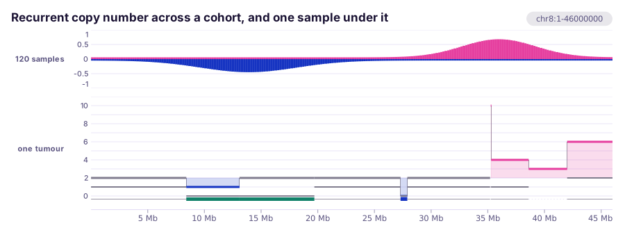
Show how often each stretch of a chromosome is gained and lost across a cohort, with no track made for it.
cargo run --example copy_number -- assets.use karyon::{plot, QuantitativeAxis, Window, WindowTrack};
// `gained` and `lost` hold, for each 100 kb span in turn, the fraction of the
// cohort in which it was gained and the fraction in which it was lost.
let mut landscape = Vec::new();
for (i, (gain, loss)) in gained.iter().zip(&lost).enumerate() {
let from = i as u64 * 100_000;
landscape.push(Window::new(from, from + 100_000, *gain));
landscape.push(Window::new(from, from + 100_000, -loss));
}
plot("chr8:1-4,000,000")?
.add_track(
WindowTrack::new(landscape)
// Warm for gained and cool for lost, the field's convention and
// the other way round from the default.
.colors("#d55e00", "#0072b2")
.axis(QuantitativeAxis::new().range(-1.0, 1.0).ticks(3))
.label("120 samples"),
)
.save("landscape.svg")?;
A window track already draws this, because nothing limits it to one row per place: here there are two over every span, gains up and losses down. Each row is a fraction rather than a count, so the axis reads the same whatever the size of the cohort.
Why two rows rather than one net value
A stretch gained in half the cohort and lost in a quarter of it nets to the same value as one gained in a quarter and never lost. Kept as two rows, both show: where several windows share a pixel column, the track keeps the lowest and the highest value in it and draws both, so a stretch that went both ways is drawn going both ways at any zoom.
A locus in detail
A locus from the files a pipeline already wrote
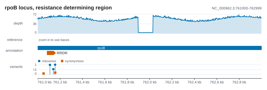
Stack depth, reference, annotation and calls over one locus, straight from the files on disk.
cargo run --example locus -- assets.karyon chr7:140,753,000-140,754,000 \
--coverage depth.bedgraph --label depth --aggregate min \
--sequence chr7.fa \
--features genes.gff3 --label annotation \
--variants calls.vcf --label variants \
--title 'BRAF exon 15' -o braf.svg
Each track flag starts a track and the options after it describe that one, so
the order of the flags is the order of the stack. --aggregate min because
when a pixel column covers several bases, a dropout is the thing worth
keeping; the default is max. The ruler goes on the bottom without being
asked for.
What --sequence takes
The record of the FASTA named like the region's sequence, or the file's
only record, cut to the region by position, so it has to be the whole
sequence the region is on. A file of several records is searched by name
and read whole: cut the one you want out first, for example with
samtools faidx genome.fa chr7 > chr7.fa, to save reading the rest.
Zooming to base resolution
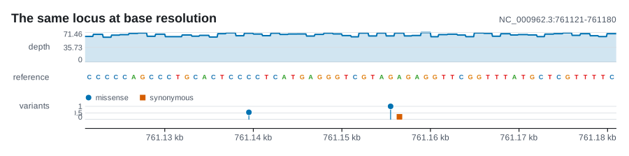
Show the same tracks over a few dozen bases, where every base has its letter.
use karyon::plot;

// `depth` and `bases` cover NC_000962.3:761,000-762,999, so their first
// value sits at 0-based 760,999. The zoom starts at 761,121 in the locus
// string, which is 761,120 counting from 0.
let offset = (761_120 - 760_999) as usize;

plot("NC_000962.3:761,121-761,180")?
    .title("Sixty bases")
    .add_coverage(depth[offset..offset + 60].to_vec())
    .label("depth")
    .add_sequence(bases[offset..offset + 60].to_vec())
    .label("reference")
    .save("zoom.svg")?;
Only the region changes. add_coverage and add_sequence start their arrays
at the left edge of the region, which is why the slices have to line up with
it; add_coverage_at and add_sequence_at take a start of their own. On the
command line nothing has to line up, because every file carries its own
coordinates. The sequence track follows the zoom the way a genome browser
does: a letter per base while a base is at least 7 pixels wide, coloured
blocks down to 0.6 of a pixel, and below that a hint to zoom in rather than a
smear of rectangles.
The reads themselves, when a call looks wrong
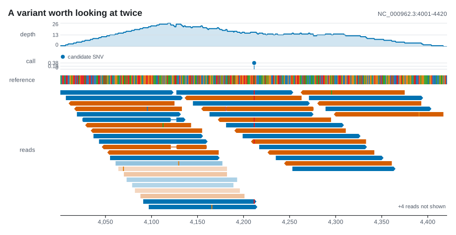
Look at the aligned reads under a call, with every base that disagrees with the reference painted.
cargo run --example pileup -- assets, with the reference attached.use karyon::{plot, ReadColoring};
// `reads` is a Vec<Read>, from read::align::sam or built by hand, and
// `window` holds the reference bases of the region, the first at 0-based
// position 140,752,999.
plot("chr7:140,753,000-140,754,000")?
.add_pileup(reads)
.label("reads")
.adjust(|track| {
track
.reference(140_752_999, window) // without it, no mismatch can be found
.coloring(ReadColoring::Strand)
.fade_by_quality(true)
})
.save("reads.svg")?;
- The reader walks each read's CIGAR, so an insertion upstream does not shift
the bases after it, and keeps what the record carries:
SEQ, the strand from flag bit 16, andMAPQ. - A mismatch needs a reference to differ from:
--with-sequence(referencein Rust), or the figure's--sequencewhen the pileup is given none. With neither, every read is drawn agreeing. Like--sequence, it takes a whole-genome FASTA and picks the record the region names. --fade-by-mapq(fade_by_qualityin Rust) draws a read fainter the lower its mapping quality, and leaves its mismatches at full strength. Colouring reads by strand isReadColoring::Strand, in the library.- The pileup stops at 40 rows and counts the rest;
--max-rows alllifts the cap.
Samples and variable sites
One track per sample
Give every sample a coverage track of its own, however many there are.
use karyon::{plot, Aggregate};

// `samples` is a Vec<(String, Vec<f64>)>: a name and a depth per base.
let mut figure = plot("chr2:1-4,000")?.title("Depth across the cohort");
for (name, depth) in samples {
    figure = figure
        .add_coverage(depth)
        .label(name)
        .adjust(|track| track.height(48.0).aggregate(Aggregate::Min))
        .done();
}
figure.save("cohort.svg")?;
A plot's type names the track it is holding, and every turn of a loop has to
have the same type. done puts the pending track away and gives the plain
type back, which is also what a track added behind an if needs. On the
command line the loop only builds the list of flags, one --coverage per file
in the order the shell lists them.
Only the sites that vary
Show the columns of an alignment where the samples differ, and nothing else.
--snpscompares every record of an aligned FASTA with the first (--compare-to NAMEpicks another), keeps the columns where any record differs, gaps included, and spaces them evenly.- Evenly spaced columns are not linear in the genome, so a ruler under them
would be a lie, and none is drawn. Each column carries its own position
instead, counted from 1 like a ruler: on the command line, its column in the
alignment; in the library,
SnpTrack::offsetshifts it onto the genome. - The panel places its own columns, so the region is only a label here.
--traits sheet.tsvdraws what is known about each sample as strips beside the rows, and--max-rowssets how many rows are drawn before the rest are counted.
A tree beside the variable sites
Sort the samples by a phylogeny, so that a clade's shared differences line up into a block.
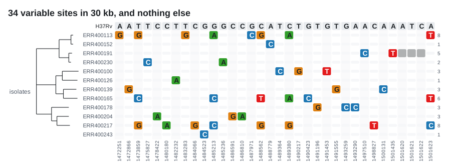
cargo run --example snps -- assets.use karyon::tree::Tree;
use karyon::{Figure, Region, SnpTrack};
let tree =
Tree::parse_newick("((ERR01:0.01,ERR02:0.012)0.98:0.04,(ERR03:0.02,ERR04:0.03):0.05);")?;
// Row 0 of the alignment is the reference the sites are called against.
let panel = SnpTrack::from_alignment(0, &alignment)
.offset(1_472_000)
.tree(tree)
.label("isolates");
// The axis counts sites, not bases, so the region is as wide as the panel
// has columns.
let region = Region::new("sites", 0, panel.sites().len() as u64)?;
Figure::new(region)
.title(format!("{} variable sites", panel.sites().len()))
.show_region_label(false)
.push(panel)
.save_svg("sites.svg")?;
This is the case Figure is for: the track is read before it is drawn,
because panel.sites() sizes the region. alignment is a Vec<MsaSequence>,
for example the records read::seq::alignment returns, each turned into
MsaSequence::new(name, residues). Rows are matched to leaves by name, and a
sample the tree does not mention keeps its place at the bottom rather than
vanishing.
The figure carries one more thing than the code: three strips of sample
metadata between the names and the panel, attached with .traits(..) from a
sample sheet (see SnpTrack). Lineage runs in
three blocks, because a lineage is inherited and the tree put the rows in that
order. Resistance does not, and that is the finding: the same phenotype in two
clades that did not inherit it from each other.
Association and whole genomes
An association scan and the genotypes under it
Put a Manhattan plot over the genotypes of the samples at the sites it tested.
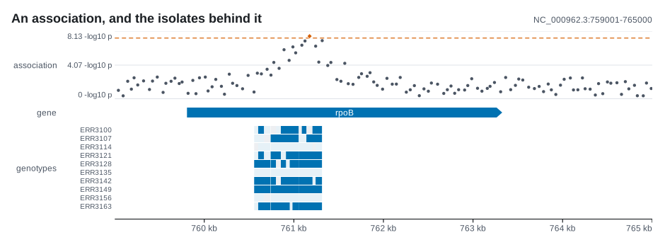
cargo run --example association -- assets.karyon chr1:1,000-2,000 \
--manhattan scan.tsv --label association \
--matrix genotypes.tsv --label genotypes \
-o association.svg
scan.tsv holds a position and a value on each line, optionally with a
sequence name in front, and may start with a header naming its columns. A
column headed as p-values are, P, pvalue or p_wald, is drawn as -log10
of itself, and any other value as written, a -log10(p) included. An
association tool's own table, PLINK's or REGENIE's with all its columns, is
read by its header as it is.
genotypes.tsv has the site positions across its header and a sample name at
the start of every row. Positions are 1-based in both, the way association
tools write them.
A cell that is empty, . or NA is missing and gets a grey of its own,
because zero is a genotype and the two have to look different. There is no
significance line until you ask for one: --threshold takes a value in the
file's units, or genome-wide for -log10(5e-8), which assumes a million
independent tests.
A scan across a whole assembly
Lay the contigs of an assembly end to end and plot a scan across all of them at once.
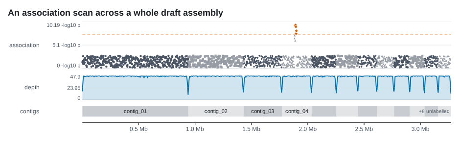
cargo run --example genomewide -- assets.use karyon::{Association, Genome, Plot};
let genome = Genome::checked([
("contig_01", 900_000u64),
("contig_02", 460_000),
("contig_03", 310_000),
])?;
// The scan reports per contig, in its own coordinates. Anything the genome
// cannot place is counted rather than dropped in silence.
let (mapped, dropped) = genome.map(hits);
eprintln!("{dropped} points could not be placed on the assembly");
let points: Vec<Association> = mapped
.iter()
.map(|(at, value)| Association::new(*at, *value))
.collect();
Plot::over(genome.region())
.title("An association scan across a draft assembly")
.remove_region_label()
.add_manhattan(points)
.label("association")
.adjust(|track| {
track
.bands(genome.boundaries())
.genome_wide_threshold()
.axis_title("-log10 p")
})
.add_genome(genome)
.label("contigs")
.save("scan.svg")?;
hits yields (String, u64, f64): the sequence name, the 0-based position on
it, and the value. Genome::map places each one on the shared axis and counts
what it could not place, a name the genome lacks or a position past the end of
its sequence, rather than drawing it somewhere plausible. Genome::checked
refuses two sequences with the same name, since Genome::at would otherwise
put everything on the first of them. bands alternates the shade of the
points at each boundary, and add_genome draws the contigs underneath.
genome_wide_threshold is a convention, not a result
It is the Bonferroni correction for a million independent tests: the
convention in human GWAS, and often the wrong number elsewhere. A shorter
genome or stronger linkage leaves far fewer than a million. Use
threshold when you know yours.
Trees
Support, branch events and distance on one phylogram
Show support, the changes on each branch and a scale of evolutionary distance on one tree.
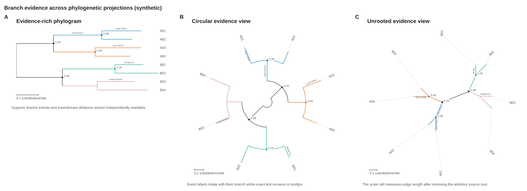
cargo run --example phylogenetics -- assets.use karyon::{Figure, Region, SupportStyle, Tree, TreeTrack};
// Support after each clade, and each node's own annotations in [&...].
let tree = Tree::parse(
"((A01[&lineage=L1,event=rpoB-S450L]:0.18,A02[&lineage=L1]:0.14)\
0.98[&lineage=L1,event=katG-S315T]:0.22,\
(B01[&lineage=L2,event=gyrA-D94G]:0.21,B02[&lineage=L2]:0.16)\
0.84[&lineage=L2]:0.19);",
)?;
Figure::new(Region::new("phylogeny", 0, 1)?)
.show_region_label(false)
.push(
TreeTrack::new(tree)
.color_by("lineage")
.support_style(SupportStyle::SymbolsAndLabels)
.support_threshold(0.70)
.branch_labels("event")
.branch_label_size(7.0)
.scale_bar_length(0.1)
.scale_bar_unit("substitutions/site"),
)
.save_svg("branch-evidence.svg")?;
color_by lets a clade take the value of its ancestor, which is right for a
lineage. branch_labels never does: an event is printed only on the branch
whose node carries it. Support written as 0.98 or as 98 is read either way, so
support_threshold(0.70) and support_threshold(70.0) both hide what is
below seventy per cent, and labels show each value as it was written. The
scale bar is in branch-length units, so it is left out of a cladogram or a
tree laid on calendar time.
To root the tree first, reroot_outgroup(["A01", "A02"]) roots it on a named
outgroup, and leaves it alone unless the names form exactly one clade;
reroot_midpoint() roots it halfway along its longest tip-to-tip path. From
the command line, --tree takes --color-by, --support-style both,
--threshold and --no-scale-bar; branch labels are in the library.
Two trees face to face
Draw two phylogenies of the same samples facing each other, so every disagreement is a crossing you can point at.
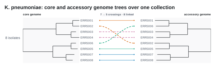
cargo run --example shapes -- assets.use karyon::{plot_tree, Tree};
let core = Tree::parse(&std::fs::read_to_string("core.nwk")?)?;
let accessory = Tree::parse(&std::fs::read_to_string("accessory.nwk")?)?;
plot_tree()
.title("Core and accessory genome trees over one collection")
.add_tanglegram(core, accessory)
.label("8 isolates")
.adjust(|track| {
track
.names("core genome", "accessory genome")
.color_by("ward")
.untangle()
})
.save("tanglegram.svg")?;
The header reports the crossings before and after untangle
(7 → 5 crossings for this pair), how many tips are linked, and how many are
unmatched when a tip is in only one tree. untangle rotates free clades and
never changes what is in them or how long their branches are. color_by
colours each tie by an annotation the two trees share, and crossing ties are
dashed, so they stay visible while colour is spent on the ward. The command
line names each tree after its file and draws both as they come; untangling
and colouring are in the library.
Why this figure has no ruler
A plot holding only phylogenies, as this one does, gets no ruler, since
nothing in it is measured in bases. remove_axis leaves the ruler out of
any other plot, and add_axis puts one exactly where you want it.
remove_region_label goes with it here, because the locus in the corner
would describe an axis that is not genomic.
Output
Dark, wide, and on standard output
Write a wide figure on a dark page to standard output, for a pipe.
Without -o the document goes to standard output, so it can be piped into
whatever converts or embeds it. The dark theme is a set of colours chosen for
a dark page, not the light one inverted: a dark background wants a narrower
band of lightness than a flipped palette lands in. karyon --help fits on one
screen, karyon help <track> lists one track's options, and
Command line is the long form.
The same stack, light and dark
Render one stack twice, once for a paper and once for a dark slide.
use karyon::{plot, Feature, Strand, Theme};

plot("chr7:140,753,000-140,754,000")?
    .title("BRAF exon 15")
    .add_coverage(depth)
    .label("depth")
    .add_features(vec![Feature::new(140_753_274, 140_753_393)
        .name("exon 15")
        .strand(Strand::Reverse)])
    .label("annotation")
    .save("braf-light.svg")?
    .theme(Theme::dark())
    .save("braf-dark.svg")?;
save writes the figure and hands the plot back, which is what lets one stack
be rendered twice. A save closes the stack: the pending track is put away and
the ruler is added, so saving twice does not draw two rulers, and a track added
after a save sits below the ruler rather than above it.
A sheet of panels
Put several figures on one sheet with letters on them, the way a paper figure is laid out.
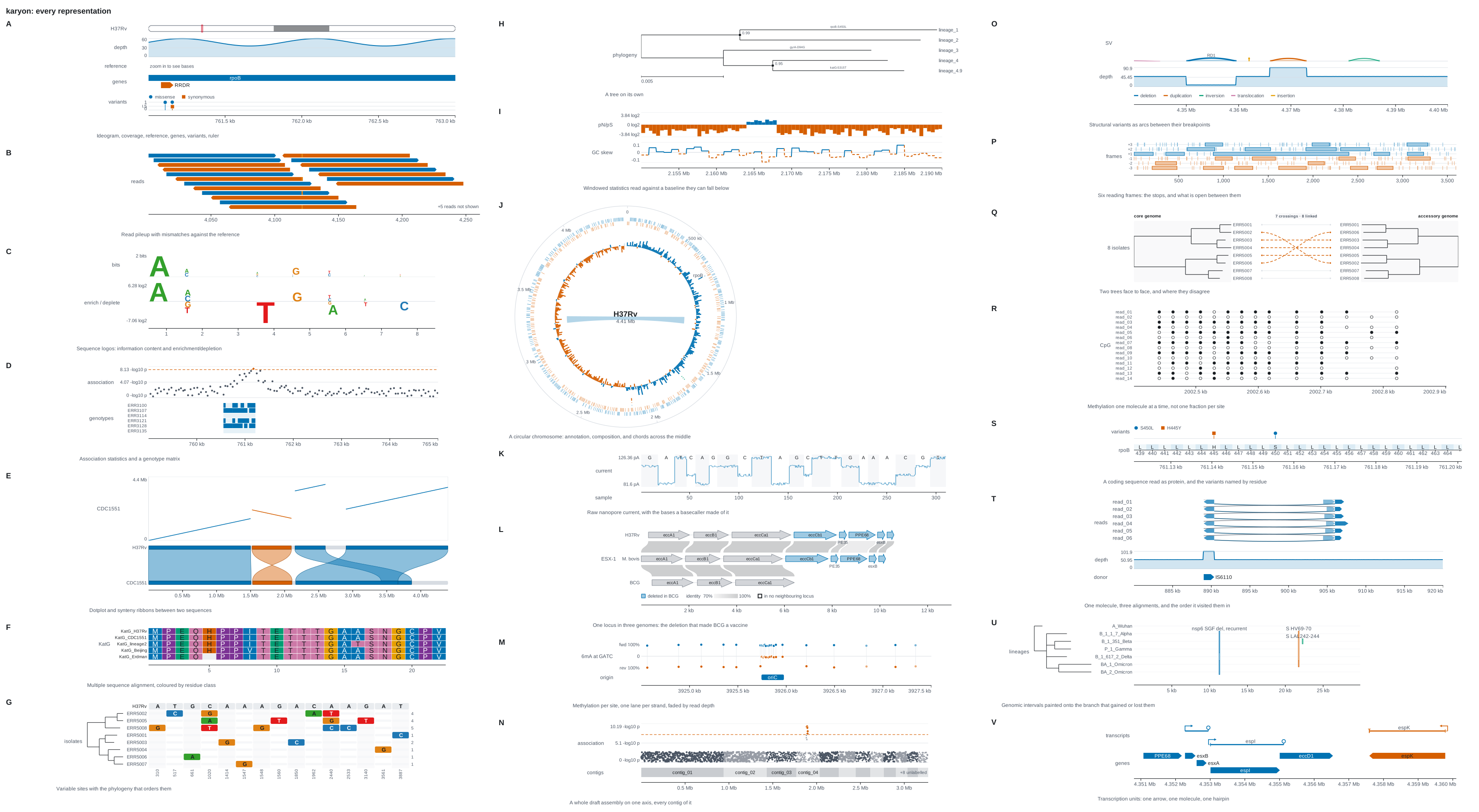
cargo run --example gallery -- assets.use karyon::{plot, Panels};
// A panel is a finished figure, which is what `into_figure` hands back.
let coverage = plot("NC_000962.3:761,000-762,999")?
.add_coverage(depth)
.label("depth")
.into_figure();
let annotation = plot("NC_000962.3:761,000-762,999")?
.add_features(genes)
.label("genes")
.into_figure();
Panels::new()
.title("Figure 1")
.columns(2)
.push_captioned(&coverage, "A", "Depth over the locus")
.push_captioned(&annotation, "B", "The annotation under it")
.save_svg("figure-1.svg")?;
Panels takes finished drawings, so a linear stack and a circular Rings
plot go on the same sheet. Panels fill each column before starting the next,
so the letters still read in order, and the column breaks are chosen to leave
the columns roughly level.
Why each panel is rendered with an id prefix
Each panel is nested whole, with a prefix on every id it generates. Ids belong to the whole SVG document, so without the prefix the second panel's clip would resolve to the first panel's rectangle and crop its tracks to somebody else's band.
One figure inside another document
Embed a figure in an HTML report next to others, without their ids colliding.
use std::io::Write;

use karyon::plot;

let figure = plot("chr1:1-1,000")?
    .add_coverage(depth)
    .label("depth")
    .add_variants(variants)
    .label("variants")
    .into_figure();

let (width, height) = figure.dimensions();
let svg = figure.to_svg_with_id_prefix("depth-");

let mut page = std::fs::File::create("report.html")?;
writeln!(
    page,
    "<figure style=\"width:{width}px\">{svg}\
     <figcaption>Depth over the first kilobase, {width} by {height} pixels.</figcaption></figure>"
)?;
to_svg is a standalone document with its own <svg> root, which is right on
disk and not inside a page that already holds figures.
to_svg_with_id_prefix puts a prefix on every id it generates, so two figures
in one document stop competing for karyon-clip-0. A prefixed figure also
leaves out its own <title> and <desc>, so say what it shows in the page
around it. The height is computed rather than set, which is why dimensions
lays the figure out to answer. Panels does the prefixing for you.
The output is plain SVG with no scripts, no external references and no
embedded fonts, so it also opens unchanged in Inkscape and Illustrator. For a
manuscript that wants PDF, figure.save_pdf("depth.pdf") writes the same
drawing as one; see How the PDF is made.
Next
-
Every track type, with its options and the files it reads.
-
Everything
plot()andFigurecan do. -
The whole grammar the shell recipes use.