Genome figures where every row lines up

One command, one figure

Name a place, then your files¶

Each file is a row, and every row is drawn on the same coordinates, so the gene, the depth over it and the calls inside it line up without anyone placing them.

A stack of four rows over two kilobases of the rpoB locus: a depth profile with a dropout in it, a reference row that says to zoom in to see bases, the gene with its resistance determining region marked inside it, variant lollipops coloured by consequence, and a coordinate ruler underneath

karyon NC_000962.3:761,000-762,999 \
  depth.bg --aggregate min reference.fa annotation.gff3 variants.vcf \
  --title 'rpoB locus, resistance determining region' \
  -o example.svg

What do you have?

Pick your data¶

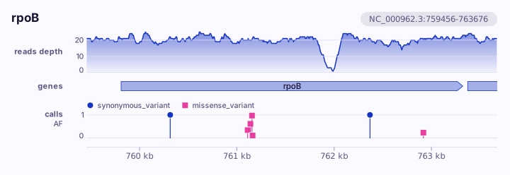
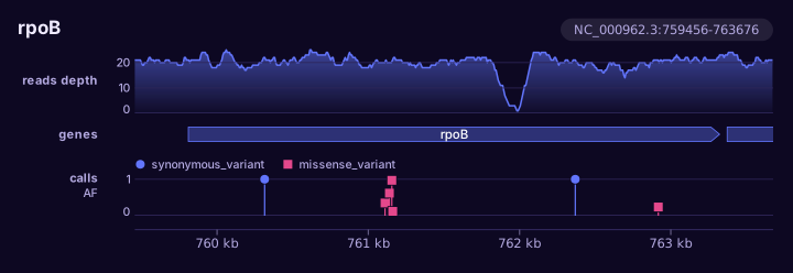
Reads, calls and genes A BAM, a VCF and an annotation over one place.
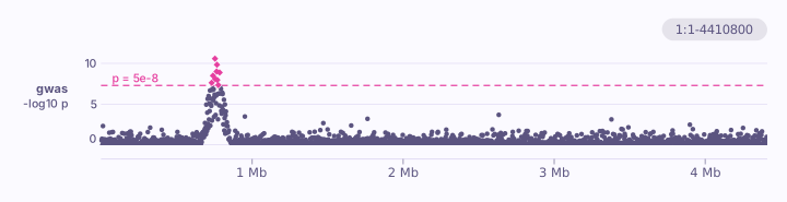
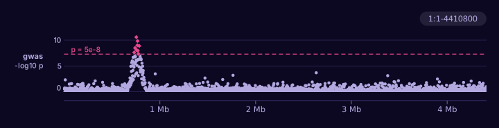
An association scan A table from PLINK, REGENIE, SAIGE or another association tool.
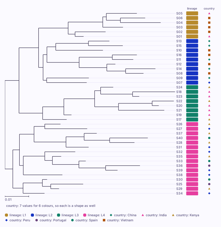
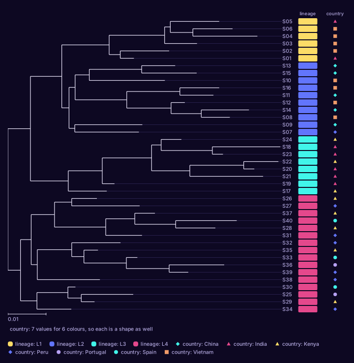
A tree and its samples A Newick tree and a sheet of what you know about each sample.
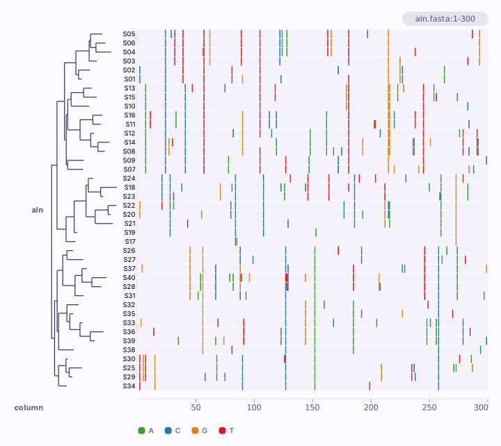
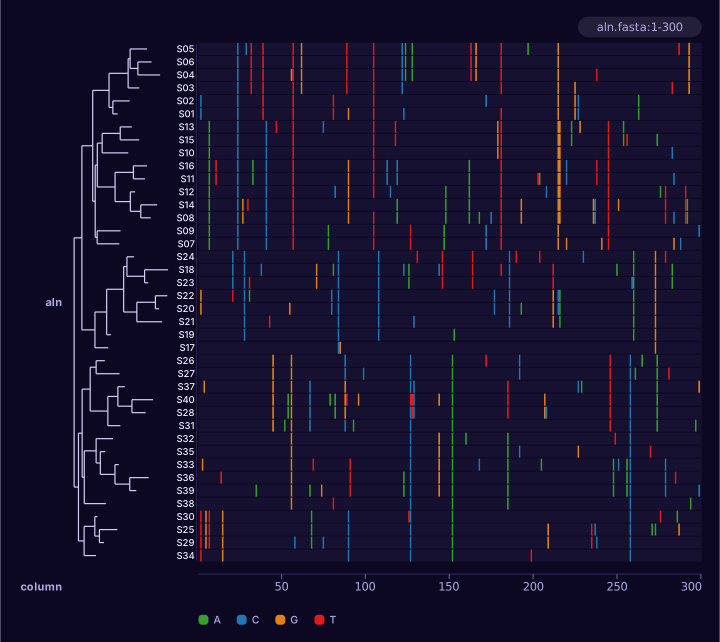
An alignment and its tree An aligned FASTA, in the order of a tree drawn beside it.
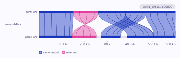
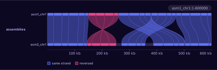
Two assemblies How two assemblies line up, from a PAF alignment.
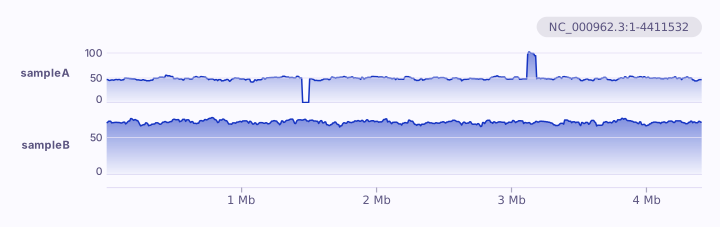
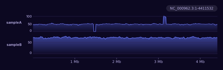
A whole sequence The depth of one sample or several along a whole chromosome.

More kinds of data Every kind of figure

Running in this page

Try it here¶

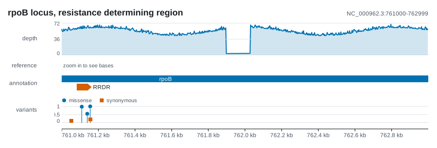
This is karyon itself, compiled to WebAssembly. Drag the figure along the genome, zoom with the buttons or the + and - keys, and watch the command above it change: every frame is a new run of it.

karyon, drawn in advance

NC_000962.3:761,000-762,999 \
  --coverage depth.bg --label depth --aggregate min \
  --features genes.gff3 --label annotation \
  --variants calls.vcf --label variants \
  --title 'rpoB locus, resistance determining region'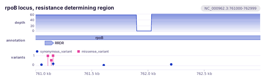

Drawn in advance from the command above. It becomes interactive once the program has loaded.

The three input files

These are the files the command reads, written out in full. Move the window somewhere none of them has data and the command answers the way it would in a terminal, for example no variants in the region, instead of drawing an empty figure.

depth.bg

NC_000962.3 756999 759999 62
NC_000962.3 759999 760999 58
NC_000962.3 760999 761899 57
NC_000962.3 761899 762029 3
NC_000962.3 762029 763999 60
NC_000962.3 763999 766999 54

genes.gff3

##gff-version 3
NC_000962.3 . gene 759807 763325 . + . Name=rpoB
NC_000962.3 . gene 761082 761162 . + . Name=RRDR

calls.vcf

NC_000962.3 760106 . C T . . AF=0.09;ANN=T|synonymous_variant|LOW|rpoB
NC_000962.3 761052 . C T . . AF=0.12;ANN=T|synonymous_variant|LOW|rpoB
NC_000962.3 761109 . G T . . AF=0.98;ANN=T|missense_variant|MODERATE|rpoB
NC_000962.3 761139 . C T . . AF=0.55;ANN=T|missense_variant|MODERATE|rpoB
NC_000962.3 761155 . T C . . AF=1.00;ANN=C|missense_variant|MODERATE|rpoB
NC_000962.3 761156 . C T . . AF=0.21;ANN=T|synonymous_variant|LOW|rpoB
NC_000962.3 761606 . G A . . AF=0.07;ANN=A|synonymous_variant|LOW|rpoB
NC_000962.3 762206 . C T . . AF=0.15;ANN=T|synonymous_variant|LOW|rpoB

Using karyon in a paper? Cite the version you used: the citation page has the reference. Built at I²SysBio, University of Valencia-CSIC, and the FISABIO Joint Research Unit Infection and Public Health, Valencia, Spain.