Comparison tracks¶

Draw one sequence against others: a multiple alignment, domain architectures side by side, two genomes as a dotplot or as ribbons, and gene neighbourhoods joined by homology.

The Rust snippets use ?, so they belong in a function that returns Result<(), Box<dyn std::error::Error>>. To choose a track by its picture, start from the gallery.

MsaTrack¶

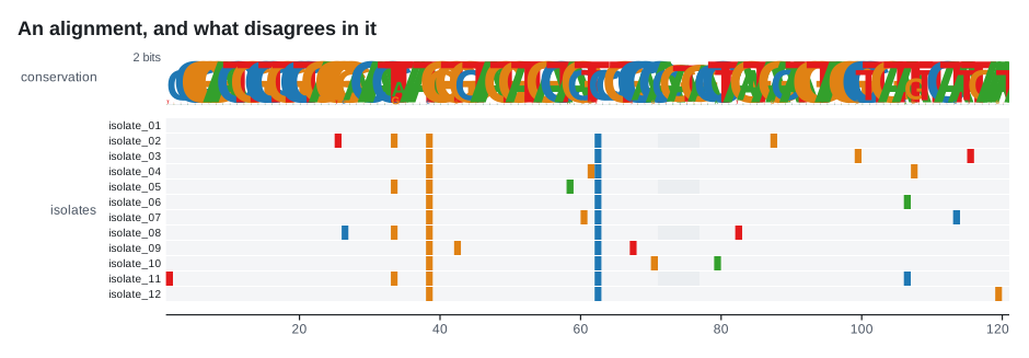
A multiple sequence alignment, row by row, painting only what disagrees with the consensus or with a row you name. In a real alignment most cells agree, and the agreement is the noise.

A conservation logo above a multiple sequence alignment, with only the disagreements painted


Rust	`.add_msa(sequences)` on `plot()`; `MsaTrack::new(sequences)`
Command line	`--msa FILE`, with `--compare-to`, `--style`, `--row-height`, `--max-rows`, `--no-names`, `--traits`, `--columns`
Reads	aligned FASTA, every record the length of the first (`read::seq::alignment`)

RustCommand line

use karyon::{plot_alignment, MsaSequence};

let rows = vec![
    MsaSequence::new("H37Rv", b"ACGTACGTAC".to_vec()),
    MsaSequence::new("CDC1551", b"ACGTTCGTAC".to_vec()),
    MsaSequence::new("Beijing", b"ACGT-CGTAC".to_vec()),
];

plot_alignment(rows)
    .label("isolates")
    .adjust(|track| track.compare_to(0))
    .save("msa.svg")?;

karyon alignment:1-120 --msa isolates.fa --compare-to H37Rv --label isolates -o msa.svg

Options¶

Method	What it does	Default
`.label("isolates")`	Names the track in the left gutter (`--label`)	none
`.row_height(14.0)`	Height of one row (`--row-height`)	`12`
`.row_gap(2.0)`	Gap between rows	`1`
`.display(MsaDisplay::Bases)`	`Differences` only, or every residue with `Bases` (`--style differences` or `all`)	`Differences`
`.coloring(MsaColoring::Residue)`	What a colour means: `Nucleotide`, `Residue` (six amino acid classes) or `Uniform`	`Nucleotide`
`.compare_to(0)`	Reads every row against this row instead of the consensus (`--compare-to NAME`)	the consensus
`.max_rows(Some(100))`	Caps the rows drawn; `None` lifts the cap (`--max-rows`)	`Some(40)`
`.show_names(false)`	Shows or hides sequence names (`--no-names`)	shown
`.show_letters(false)`	Shows or hides residue letters once a column is wide enough	shown
`.match_color("#e5e7eb")`	Colour of a cell that agrees with the comparison row	from the theme
`.gap_color("#9ca3af")`	Colour of a gap	from the theme
`.uniform_color("#d55e00")`	Colour of every difference under `Uniform`	theme accent
`.tree(tree)`	Draws a phylogeny beside the rows and sorts them by descent	none
`.tree_width(120.0)`	Width of the tree strip in pixels	`100`
`.tree_shape(TreeShape::Cladogram)`	Phylogram or cladogram for that tree	`Phylogram`
`.traits(traits)`	Metadata columns between the names and the rows (`--traits`, `--columns`)	none

Notes¶

The coordinates are alignment columns, not genomic positions, so the figure's region is the column space: an alignment 900 columns wide is plot("alignment:1-900"), and the ruler under it counts columns. Ungapping a row back to reference coordinates is a real operation with real decisions in it, and the crate does not do it behind your back.

Which row the others are read against matters as much as the display. It is the consensus until compare_to names one; ties in the consensus go to the residue seen first, so it never changes between runs. On the command line, --compare-to takes the name in the FASTA header and refuses a name that is missing or repeated.

Conservation belongs above the alignment rather than inside it: a LogoTrack built with LogoTrack::from_sequences takes the same sequences. Rows are capped at forty and what the cap hid is counted in the corner, and runs of equally coloured cells are merged into one rectangle, which is what keeps a wide alignment from becoming a file no viewer will open.

A protein alignment wants .coloring(MsaColoring::Residue): six physicochemical classes, as many as the validated palette has hues, with glycine and proline in classes of their own.

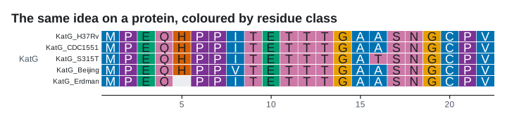
A short protein alignment with residues coloured by class

tree matches sequence names to leaves, sorts the rows by descent and draws the tree in the name strip. A chosen comparison row follows its sequence when the rows move, and sequences the tree does not name stay at the bottom rather than being dropped.

DomainTrack¶

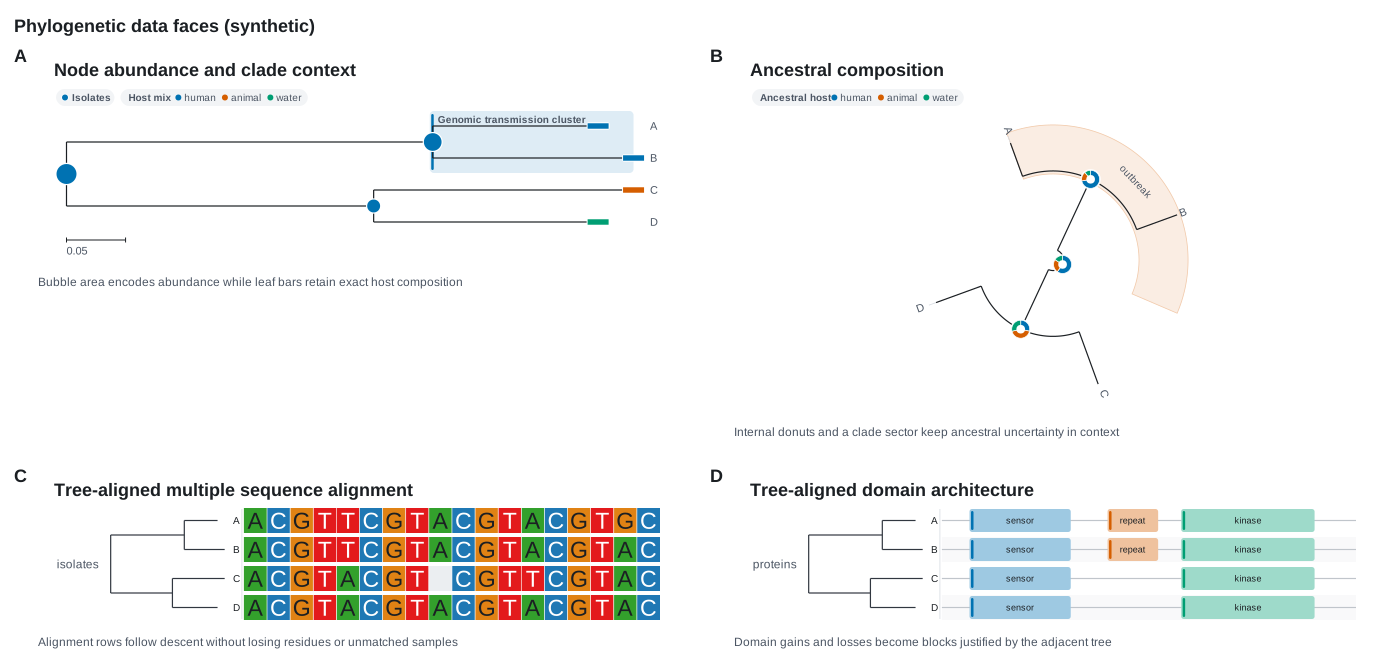
Domains, motifs, exons or repeats as labelled intervals along a protein or transcript, one sequence per row, so gains, losses and rearrangements of architecture can be read against each other.

Domain architectures in rows sorted by the phylogeny beside them, so domain gains and losses come out as blocks, in a sheet with an alignment sorted the same way and two trees carrying bubbles, bars and ancestral-state donuts


Rust	`.add_domains(rows)` on `plot()`; `DomainTrack::new(rows)`
Command line	`--domains FILE`, with `--analysis`, `--row-height`, `--no-names`, `--traits`, `--columns`
Reads	an `InterProScan` table (`read::domain::architectures`)

RustCommand line

use karyon::{plot, DomainArchitecture, DomainFeature};

plot("protein:1-500")?
    .add_domains(vec![
        DomainArchitecture::new("P1", 500)
            .feature(DomainFeature::new(10, 275).label("Protein kinase"))
            .feature(DomainFeature::new(340, 400).label("PASTA")),
        DomainArchitecture::new("P2", 420)
            .feature(DomainFeature::new(19, 280).label("Protein kinase")),
    ])
    .label("domains")
    .save("domains.svg")?;

karyon P1:1-500 --domains interpro.tsv --analysis Pfam --label Pfam -o domains.svg

Options¶

Method	What it does	Default
`.label("domains")`	Names the track in the left gutter (`--label`; the command line uses the analysis when there is none)	none
`.row_height(18.0)`	Height of one architecture row (`--row-height`)	`14`
`.row_gap(4.0)`	Gap between rows, in the page colour	`3`
`.show_names(false)`	Shows or hides sequence names (`--no-names`)	shown
`.show_labels(false)`	Shows or hides domain names inside intervals wide enough to hold them	shown
`.tree(tree)`	Draws a phylogeny beside the rows and sorts them by descent	none
`.tree_width(120.0)`	Width of the tree strip in pixels	`100`
`.tree_shape(TreeShape::Cladogram)`	Phylogram or cladogram for that tree	`Phylogram`
`.traits(traits)`	Metadata columns between the names and the rows (`--traits`, `--columns`)	none

Notes¶

A domain is at a place in a protein, so the axis is residues: the region is a residue range, as in P00533:1-1,210, and the ruler counts amino acids. Intervals are 0-based and half-open like every other interval in the crate; InterProScan's 1-based start comes back one lower.

Features with the same label share one palette colour across rows, so one domain family is one colour everywhere, and DomainFeature::color overrides it when a source already defines colours. Names are drawn only where they fit; the tooltips keep the full name and exact boundaries.

Column one of an InterProScan table names the row rather than selecting it, so every protein in the file is drawn on one shared axis, and a protein with no domain is still a row with its backbone. --analysis picks one member database, such as Pfam or PANTHER, from a file where several describe the same protein; the command refuses to choose for you.

tree matches architecture names to leaves and reorders the rows by descent, drawing the tree in the name strip; rows the tree does not name stay at the bottom. Unlike a TreeTrack, the horizontal axis is still the sequence coordinate.

DotplotTrack¶

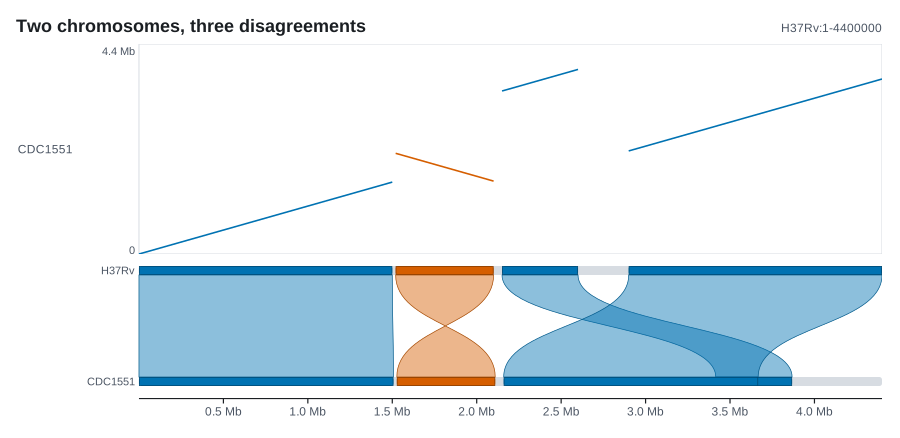
Two sequences on two axes, with each alignment block drawn as a diagonal. A forward block runs up to the right and a reversed one down, so a rearrangement has a shape: a translocation sits off the main diagonal and an inversion is an anti-diagonal.

A dotplot above a ribbon plot of the same two chromosomes, showing a colinear region, an inversion as an anti-diagonal and a crossed ribbon, and a translocated block


Rust	`.add_dotplot(blocks)` on `plot()`; `DotplotTrack::new(blocks)`
Command line	`--dotplot FILE`, with `--height`
Reads	PAF, as `minimap2` writes it (`read::align_pairs::blocks`)

RustCommand line

use karyon::{plot, AlignmentBlock};

let blocks = vec![
    AlignmentBlock::new(0, 1_400_000, 0, 1_398_000),
    AlignmentBlock::new(1_400_000, 2_250_000, 1_398_000, 2_248_000).reversed(true),
];

plot("H37Rv:1-4,411,532")?
    .add_dotplot(blocks)
    .label("CDC1551")
    .adjust(|track| track.target_length(4_403_837))
    .save("dotplot.svg")?;

karyon H37Rv:1-4,411,532 --dotplot H37Rv-CDC1551.paf --label CDC1551 -o dotplot.svg

Options¶

Method	What it does	Default
`.label("CDC1551")`	Names the track in the left gutter (`--label`)	none
`.height(260.0)`	Band height in pixels; a dotplot wants to be tall (`--height`)	`190`
`.target_length(4_403_837)`	Puts the whole target on the vertical axis	what the blocks reach
`.target_range(1_000_000, 2_000_000)`	Puts one span of the target on the vertical axis	what the blocks reach
`.forward_color("#0072b2")`	Colour of forward blocks	from the theme
`.reverse_color("#d55e00")`	Colour of reversed blocks	from the theme
`.line_width(2.0)`	Stroke width of a diagonal	`1.6`
`.show_frame(false)`	Shows or hides the box around the panel	shown
`.show_scale(false)`	Shows or hides the target coordinate labels	shown

Notes¶

The figure's region is always the query; the target keeps a scale of its own on the vertical axis. Left unpinned, that axis spans exactly what the blocks reach, so two lists differing by one block are two different axes and neither says so. Fix it with target_length or target_range whenever two figures are meant to be read against each other.

An AlignmentBlock keeps both spans ascending and the strand as a flag, reversed(true), which is how PAF records them; PAF is already 0-based and half-open, so nothing is converted.

A PAF names both sequences on every row. From the command line the query is the sequence the region names, the target is the one with the most alignments to it, and the target length comes from the file.

SyntenyTrack¶

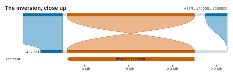
The same alignment blocks as ribbons between two bars: the compact form of the comparison, which sits in a stack of other tracks and turns an inversion into a twist.

The inversion on its own: two bars joined by ribbons that cross where the alignment reverses


Rust	`.add_synteny(blocks)` on `plot()`; `SyntenyTrack::new(blocks)`
Command line	`--synteny FILE`, with `--height`
Reads	PAF (`read::align_pairs::blocks`); the most-aligned target is drawn and both sequences are named

RustCommand line

use karyon::{plot, AlignmentBlock};

let blocks = vec![
    AlignmentBlock::new(0, 1_400_000, 0, 1_398_000),
    AlignmentBlock::new(1_400_000, 2_250_000, 1_398_000, 2_248_000).reversed(true),
];

plot("H37Rv:1-4,411,532")?
    .add_synteny(blocks)
    .adjust(|track| track.target_length(4_403_837).names("H37Rv", "CDC1551"))
    .save("synteny.svg")?;

karyon H37Rv:1-4,411,532 --synteny H37Rv-CDC1551.paf -o synteny.svg

Options¶

Method	What it does	Default
`.label("CDC1551")`	Names the track in the left gutter (`--label`)	none
`.height(140.0)`	Band height in pixels (`--height`)	`110`
`.bar_height(12.0)`	Thickness of the two sequence bars	`9`
`.target_length(4_403_837)`	Puts the whole target on the lower bar	what the blocks reach
`.target_range(1_000_000, 2_000_000)`	Puts one span of the target on the lower bar	what the blocks reach
`.names("H37Rv", "CDC1551")`	Names the two sequences beside their bars	none; the command line names both
`.forward_color("#0072b2")`	Colour of forward ribbons	from the theme
`.reverse_color("#d55e00")`	Colour of reversed ribbons	from the theme
`.ribbon_opacity(0.6)`	How solid a ribbon is, from 0 to 1	`0.45`

Notes¶

Neither form is a summary of the other, which is why both exist. A DotplotTrack shows the shape of a rearrangement at a glance and costs a tall panel; the ribbons cost one band, follow one block at a time, and stay in register with the coverage and annotation stacked around them.

Ribbons are translucent, so two crossing ones read as two and a pile of them shows that it is a pile, and each block is also drawn solid on both bars, so a thin ribbon still shows exactly what it connects. As with the dotplot, pin the target with target_length or target_range when two figures are compared.

LocusTrack¶

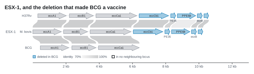
Several loci from several genomes, one row each, genes drawn as arrows and joined to their matches in the row below by ribbons shaded by identity. Genes that match nothing are outlined, because what one locus has and the other has not is usually the question.

The ESX-1 locus in three genomes, one row each, genes drawn as arrows and joined by identity ribbons, with the genes deleted in one of them left outlined and unjoined


Rust	`.add_loci(loci)` on `plot()`, then `.links(homologies)`; `LocusTrack::new(loci)`
Command line	`--loci FILE --links FILE`, with `--identity`, `--no-names`, `--traits`, `--columns`, `--format`
Reads	BED or GFF3 whose first column names the genome (`read::locus::loci`), and BLAST tabular output or two or three columns of gene names (`read::locus::links`)

RustCommand line

use karyon::{plot, Feature, Homology, Locus, Strand};

let loci = vec![
    Locus::new(
        "H37Rv",
        vec![
            Feature::new(300, 2_022).name("eccA1").strand(Strand::Forward),
            Feature::new(8_700, 9_807).name("PPE68").strand(Strand::Forward),
        ],
    ),
    Locus::new("BCG", vec![Feature::new(300, 2_022).name("eccA1").strand(Strand::Forward)])
        .offset(150),
];

plot("ESX-1:1-10,000")?
    .add_loci(loci)
    .label("ESX-1")
    .adjust(|track| track.links(vec![Homology::new(0, 0, 0, 0.999)]))
    .save("esx1.svg")?;

karyon ESX-1:1-10,000 --loci loci.bed --links hits.tsv --label ESX-1 -o esx1.svg

Options¶

Method	What it does	Default
`.links(homologies)`	The homologies between neighbouring rows (`--links`)	none
`.label("ESX-1")`	Names the track in the left gutter (`--label`)	none
`.gene_height(26.0)`	Height of one gene	`22`
`.link_height(40.0)`	Room the ribbons get between two rows	`34`
`.show_names(false)`	Shows or hides the genome names (`--no-names`)	shown
`.show_gene_names(false)`	Shows or hides gene names, where there is room	shown
`.colors(forward, reverse)`	Colours of forward and reverse genes without their own	the strand colours
`.min_gene_width(3.0)`	Narrowest a gene is drawn, in pixels	`2`
`.shape(GeneShape::Pointed)`	`Arrow`, a shaft with an overhanging head, or `Pointed`, for short genes	`Arrow`
`.soft_fills(false)`	Draws each gene as a wash of its colour edged in the colour, or in the colour as given	on
`.link_inset(6.0)`	Gap between a gene and the ribbon leaving it, in pixels	`4`
`.mark_unmatched(false)`	Outlines the genes no homology reaches	on
`.identity_range(0.8, 1.0)`	Identities mapped to the palest and darkest ribbon	`0.7` to `1.0`
`.traits(traits)`	Metadata columns between the genome names and the loci (`--traits`, `--columns`)	none

Notes¶

The question asked of a gene cluster, an operon or a viral genome is rarely what is in it, and usually what is in it that the other one has not. The missing ribbon says so only to a reader who thought to look for an absence, so mark_unmatched outlines those genes by default; unmatched(row) lists them.

The x axis is the figure's own, so a kilobase is a kilobase in every row and loci can be compared for length as well as content. Give each Locus its genes in the coordinates they came in, and line a row up with its neighbour with Locus::offset.

Homology::new(row, from, to, identity) joins gene from of row to gene to of the row below, and homologies join neighbouring rows only: a ribbon that skips a row crosses one it has nothing to do with. Homology::unstated is a match with no number on it, drawn at the pale end and outlined. Set identity_range to the range the data occupies, since orthologues sit between about seventy and a hundred per cent and a ramp from nought to one draws them all alike. ramp_ends(&theme) hands the two ends of the shading to a LegendTrack.

The join from a links file is by gene name, and the command line refuses a file whose names join nothing, because every gene outlined reads as a discovery rather than as a mistake. --identity percent or fraction settles a third column that could be either.