Signal and sequence tracks¶

Draw what a sequence carries base by base: a depth profile, a statistic in windows, methylation on each strand, the bases themselves, a sequence logo, or the bases a model leaned on.

The Rust snippets use ?, so they belong in a function that returns Result<(), Box<dyn std::error::Error>>, and names such as depth stand for data you already hold. To choose a track by its picture, start from the gallery.

CoverageTrack¶

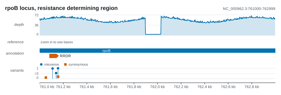
A quantity with one value per base, drawn up from the floor of its band: read depth, GC content, mappability. Use it for anything whose zero is a real bottom.

A depth profile across two kilobases of rpoB with a dropout in it, drawn with the minimum of each pixel column, above the reference, the gene and its variants


Rust	`.add_coverage(values)` or `.add_coverage_at(start, values)` on `plot()`; `CoverageTrack::new(start, values)`, `CoverageTrack::from_spans(&region, spans)`, `CoverageTrack::from_pairs(&region, pairs)`
Command line	`--coverage FILE`, with `--aggregate`, `--style`, `--log`, `--color`, `--height`, `--format`; `--recombination FILE` draws a recombination rate as a line in cM/Mb
Reads	bedGraph, `samtools depth`, one value per line, or a BAM, whose depth it counts as `samtools depth -a` does (`read::signal::spans`, `read::bam`); a genetic map as HapMap writes one (`read::recombination::rates`)

RustCommand line

use karyon::{plot, Aggregate};

// depth: Vec<f64>, one value per base from the left edge of the region
plot("NC_000962.3:761,001-763,000")?
    .add_coverage(depth)
    .label("depth")
    .adjust(|track| track.aggregate(Aggregate::Min).height(70.0))
    .save("depth.svg")?;

karyon NC_000962.3:761,001-763,000 \
  --coverage depth.bedgraph --label depth --aggregate min --height 70 \
  -o depth.svg

Options¶

Method	What it does	Default
`.label("depth")`	Names the track in the left gutter (`--label`)	none
`.height(70.0)`	Band height in pixels (`--height`)	`60`
`.aggregate(Aggregate::Min)`	How a pixel column covering many bases is reduced: `Max`, `Mean` or `Min` (`--aggregate`)	`Max`
`.style(CoverageStyle::Line)`	`Area`, `Line` or `Bars` (`--style area`, `line` or `bars`)	`Area`
`.axis_title("cM/Mb")`	What the value axis measures, under the track's name	none; `cM/Mb` from `--recombination`
`.max(120.0)`	Pins the top of the axis, taken literally	the largest value on screen, plus six per cent
`.log_scale(true)`	Plots `log10(1 + value)`, still labelled in the original units (`--log`)	off
`.color("#0072b2")`	Colour of the profile (`--color`)	theme accent
`.fill_opacity(0.4)`	Fill opacity, from 0 to 1	`0.18` for an area, solid for bars
`.show_max(false)`	Shows or hides the small maximum-value note	shown
`.axis(QuantitativeAxis::new().range(0.0, 100.0))`	Replaces the value axis: range, ticks, unit, reference lines	automatic

Notes¶

When a pixel covers many bases, the aggregate is a claim about what you are looking for. Max, the default, keeps a one-base spike visible across a megabase, which is what you want when hunting duplications; across the same view it draws a 300 bp deletion flat. Min shows the dropout. Whatever the region, the SVG holds at most one point per pixel column.

The ceiling moves with the view unless it is pinned, so pin max whenever two samples sit side by side, or the eye reads two scales as one. log_scale is the other way to fit a thousandfold range into one band.

CoverageTrack::new draws only the values it holds: bases outside them are not drawn, and non-finite values are missing, so a gap in the input stays a gap. from_spans and from_pairs span the region, not the genome, and leave every base they are not given at nought, which is what a bedGraph means by leaving it out. The command line reads the same way.

A profile is kept as runs of bases holding one value, so what it costs follows how often the value changes, not how long the region is. A bedGraph of windows over 200 Mb is a few thousand runs: a value per base made it 1.6 GB, and it now takes 4 MB. A per-base depth file changes value at almost every base and costs what it did.

The profile rises from the floor of the band, which says that zero is the bottom. That is true of read depth and false of a signed or centred statistic: a number that can fall below its baseline belongs in a WindowTrack.

WindowTrack¶

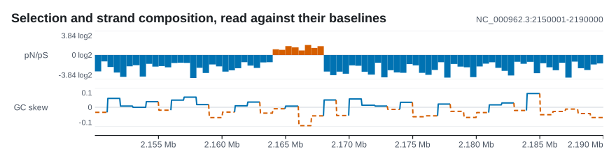
A statistic computed in windows, drawn either side of a baseline it can fall below: pN/pS centred on one, GC skew and Tajima's D centred on nought. Use it when which side of the line a window falls on is the point.

pN/pS and GC skew in windows along forty kilobases, each drawn either side of its own baseline, with the windows below the line in a colour of their own


Rust	`.add_windows(windows)` on `plot()`; `WindowTrack::new(windows)`, `WindowTrack::ratios(windows)`, `WindowTrack::gc_skew(start, &seq, window)`, `WindowTrack::gc_content(start, &seq, window)`
Command line	`--windows FILE`, with `--style`, `--height`
Reads	bedGraph, one window per row (`read::signal::windows`)

RustCommand line

use karyon::{plot, Window, WindowTrack};

let pnps = vec![
    Window::new(2_150_000, 2_160_000, 0.42),
    Window::new(2_160_000, 2_170_000, 2.10),
    Window::new(2_170_000, 2_180_000, 0.85),
    Window::new(2_180_000, 2_190_000, 1.30),
];

// bases: Vec<u8>, the sequence of the region from 0-based 2,150,000
plot("NC_000962.3:2,150,001-2,190,000")?
    .add_track(WindowTrack::ratios(pnps).label("pN/pS"))
    .add_track(WindowTrack::gc_skew(2_150_000, &bases, 1_000).label("GC skew"))
    .save("selection.svg")?;

karyon NC_000962.3:2,150,001-2,190,000 \
  --windows gc-skew.bedgraph --label 'GC skew' --style line \
  -o skew.svg

Options¶

Method	What it does	Default
`.label("pN/pS")`	Names the track in the left gutter (`--label`)	none
`.height(80.0)`	Band height in pixels (`--height`)	`56`
`.baseline(1.0)`	Moves the line the statistic is read against	`0`, or the genome's own GC content for `gc_content`
`.style(WindowStyle::Line)`	`Steps`, a block per window, or `Line` (`--style steps` or `line`)	`Steps`
`.colors("#d55e00", "#0072b2")`	Colours of windows above and below the baseline	from the theme
`.extent(3.0)`	Pins how far the axis reaches either side of the baseline	every window's range
`.symmetric(false)`	Whether the axis reaches equally far above and below	on
`.unit(" log2")`	Suffix after each axis number	none, or `" log2"` for `ratios`
`.show_scale(false)`	Shows or hides the value axis	shown
`.axis(QuantitativeAxis::new())`	Replaces the value axis	automatic

Notes¶

Drawn up from the bottom of a band, a centred statistic loses the one thing it was computed to say. Steps is the default because a window is an interval and a block says so; Line suits a statistic read as a curve, GC skew being the usual case.

A ratio needs one more step, and WindowTrack::ratios takes it. On a linear axis a pN/pS of 0.5 sits half a unit under the line while 2.0 sits a whole unit over it; plotted as log2, the two twofold departures are the same distance away. A ratio of nought or less has no logarithm and is dropped, since a gene with no synonymous change has no ratio at all.

gc_skew and gc_content compute the statistic from the bases you hand them. gc_content puts the baseline at the GC content of the whole sequence, so a window reads as richer or poorer than its own genome rather than against an arbitrary half.

The axis range is taken over every window you pass, not only the visible ones, so panning does not rescale it. Pin extent to compare two tracks.

From the command line the baseline stays at nought, so give --windows a statistic centred on zero, or a ratio already turned into log2.

MethylationTrack¶

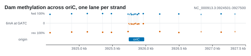
Per-site methylation, one lane per strand: forward calls above a midline and reverse calls below, each faded by how many reads it rests on. Use it for modified-base calls pooled per site, such as the output of modkit pileup.

Dam methylation at GATC sites across the E. coli origin of replication, forward strand calls above the line and reverse below, each faded by how many reads covered it


Rust	`.add_methylation(sites)` on `plot()`; `MethylationTrack::new(sites)`
Command line	`--methylation FILE`, with `--modification`, `--min-reads`, `--height`
Reads	bedMethyl from `modkit pileup` (`read::methyl::sites`)

RustCommand line

use karyon::{plot, MethylSite, MethylationTrack, Strand};

let sites = vec![
    MethylSite::new(1_010, Strand::Forward, 0.95, 40),
    MethylSite::new(1_011, Strand::Reverse, 0.08, 38),
];
let track = MethylationTrack::new(sites).min_coverage(10).label("6mA");
assert_eq!(track.hemimethylated(0.5), vec![1_010]);

plot("NC_000913.3:1,001-1,100")?.add_track(track).save("methylation.svg")?;

karyon NC_000913.3:3,924,501-3,927,500 \
  --methylation pileup.bed --modification a --min-reads 10 --label 6mA \
  -o methylation.svg

Options¶

Method	What it does	Default
`.label("6mA")`	Names the track in the left gutter (`--label`; the command line uses the modification code when there is none)	none
`.height(90.0)`	Band height in pixels (`--height`)	`76`
`.min_coverage(10)`	Drops sites called from fewer reads, and prints how many it dropped (`--min-reads`)	`5`
`.no_coverage(3)`	How many positions had no valid coverage, printed beside the floor's count; the command line passes the reader's	`0`
`.saturating_coverage(60)`	Coverage at which a site is drawn at full strength	`30`
`.pair_within(0)`	How far apart the two strands' calls of one site may sit	`1`
`.colors(forward, reverse)`	Colours of the two strands	the strand colours
`.radius(3.0)`	Radius of one site marker	`2.6`
`.show_scale(false)`	Shows or hides the fraction axis	shown
`.show_stems(false)`	Shows or hides the stem joining each marker to the midline	shown

Notes¶

A methylation call is not a variant: the base is the same base, and the measurement is a fraction of reads. Two things follow, and they are why this is not a VariantTrack.

The first is strand. Methylation belongs to one strand of a duplex, so the two strands of a palindromic site are two measurements, and the asymmetry is often the finding. The track refuses to average them. hemimethylated(by) returns the forward positions whose partner disagrees by more than by, where the partner is the nearest reverse call within pair_within: the two modified bases of a GATC or a CpG sit a base apart, never on one coordinate.

The second is coverage. A site called from four reads and one called from four hundred look the same to anything that plots the fraction alone, so sites under min_coverage are dropped, counted by discarded() and printed on the band, and the rest fade with depth up to saturating_coverage. A position with no valid coverage never becomes a site at all, since it was not measured rather than measured at 0%: read::methyl::sites skips it and counts it in Calls::no_coverage, and no_coverage(count) prints that count beside the other.

A bedMethyl from a dual-mode run holds several modification codes at one position. --modification says which to draw, and the command refuses to pick one for you when the file holds more than one.

SequenceTrack¶

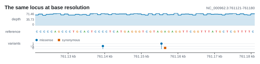
The reference bases, drawn the way a genome browser draws them: coloured letters once a base is wide enough, coloured blocks below that, and a hint to zoom in once a base is thinner than a pixel.

Sixty bases of rpoB with the reference drawn as coloured letters, between a depth profile and two variant calls


Rust	`.add_sequence(seq)` or `.add_sequence_at(start, seq)` on `plot()`; `SequenceTrack::new(start, seq)`
Command line	`--sequence FILE`, with `--height`
Reads	FASTA, its only record or the one named like the region's sequence, cut to the region (`read::seq::fasta`)

RustCommand line

use karyon::{plot, read};

let text = std::fs::read_to_string("H37Rv.fa")?;
let (_, chromosome) = read::seq::fasta(&text)?.remove(0);

plot("NC_000962.3:761,121-761,180")?
    .add_sequence_at(0, chromosome) // the whole sequence; only the region is drawn
    .label("reference")
    .save("bases.svg")?;

karyon NC_000962.3:761,121-761,180 --sequence H37Rv.fa --label reference -o bases.svg

Options¶

Method	What it does	Default
`.label("reference")`	Names the track in the left gutter (`--label`)	none
`.height(24.0)`	Band height in pixels (`--height`)	`18`
`.letter_threshold(10.0)`	Pixels a base needs before its letter is drawn	`7`
`.block_threshold(1.0)`	Pixels a base needs before any block is drawn; below it the track prints a hint	`0.6`

Notes¶

Below block_threshold the track draws nothing and prints zoom in to see bases. That is a refusal: five million one-pixel rectangles make a file no viewer will open. Above it, the cost follows the width of the figure rather than the length of the sequence, since only the bases inside the region are visited, so a whole chromosome can back a track that shows sixty bases of it.

Colours come from the theme's bases, which is BaseColors::conventional() unless you change it. Those are the colours readers expect, and adenine and guanine sit close together for a reader with protanopia; BaseColors::colorblind_safe() keeps all four apart (see Styling). Lower case is drawn as upper case, U takes the colour of T, and N or any other symbol takes one neutral grey.

While the bases are blocks, their colours name them only to a reader who knows the palette, so the command line draws a key under the figure: A, C, G and T, and other where the window holds an N. In Rust, Figure::key() gathers what every track needs explained at the zoom the figure is drawn at, and BaseColors::legend() is the key to the four colours on its own.

--sequence draws the only record of the FASTA, whatever its name, or, in a file of several, the one named like the region's sequence.

LogoTrack¶

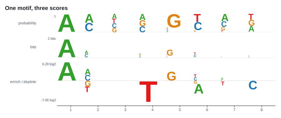
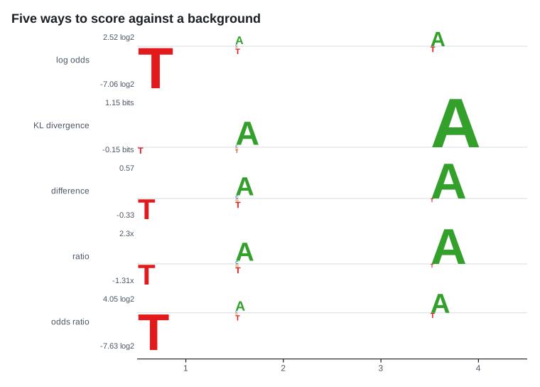
A sequence logo over consecutive positions, with seven ways to decide what a letter's height means. Five of them measure a symbol against a background and can hang it below the baseline, which a classic logo cannot do.


Rust	`.add_logo(columns)` or `.add_logo_at(start, columns)` on `plot()`; `LogoTrack::new(start, columns)`, `LogoTrack::from_sequences(start, &sequences)`, `LogoTrack::from_matrix(start, &alphabet, &columns)`
Command line	`--logo FILE`
Reads	aligned FASTA, counted column by column (`read::seq::alignment`)

RustCommand line

use karyon::{plot, LogoTrack};

let sites = ["TGACGTCA", "TGACGTCA", "TGATGTCA", "TTACGTAA", "TGACGCCA"];

plot("motif:1-8")?
    .add_track(
        LogoTrack::from_sequences(0, &sites)
            .alphabet_size(4)
            .edlogo()
            .label("motif"),
    )
    .add_axis()
    .adjust(|axis| axis.center_on_bases(true))
    .save("logo.svg")?;

karyon motif:1-8 --logo sites.fa --label motif -o logo.svg

Options¶

Method	What it does	Default
`.label("motif")`	Names the track in the left gutter (`--label`)	none
`.height(120.0)`	Band height in pixels	`80`
`.score(LogoScore::KullbackLeibler)`	What a letter's height stands for: `Probability`, `InformationContent`, `LogOdds`, `KullbackLeibler`, `Difference`, `Ratio` or `OddsRatio`	`InformationContent`
`.edlogo()`	Log odds centred on the column median, the EDLogo	off
`.centering(Centering::None)`	Where the baseline of a background-relative score sits	`Centering::median()`
`.background([("A", 0.3), ("C", 0.2), ("G", 0.2), ("T", 0.3)])`	Background frequencies the relative scores measure against	uniform
`.alphabet_size(4)`	How many symbols the alphabet has, including unseen ones	the symbols that appear
`.smoothing(0.005)`	Fraction of each column spread evenly before a log score, which bounds how far an absent symbol falls	`0.01`
`.stabilize()`	Shrinks each column towards the background by what its sample size supports	off
`.stabilize_with(dash)`	The same with a `karyon::dash::Dash` you configured	off
`.sample_size(500.0)`	Observations behind each column, for weights that are not counts	the column totals
`.max_extent(2.0)`	Pins how far the tallest stack reaches, in score units	what is on screen
`.order(StackOrder::LargestInside)`	Which end of a stack the tallest symbol takes	`LargestOutside`
`.symbol_color("A", "#009e73")`	Overrides one symbol's colour	the palette, in order of first appearance
`.min_letter_width(6.0)`	Pixels a column needs before letters are drawn; narrower columns become stacked bars	`4`
`.show_scale(false)`	Shows or hides the scale note in the corner	shown

Notes¶

A column that is nearly uniform is flat in bits, and a base missing from it is invisible. The five background-relative scores fix that by letting a symbol fall below the line; edlogo() is the one to reach for first. Which score you choose changes the reading, not just the drawing:

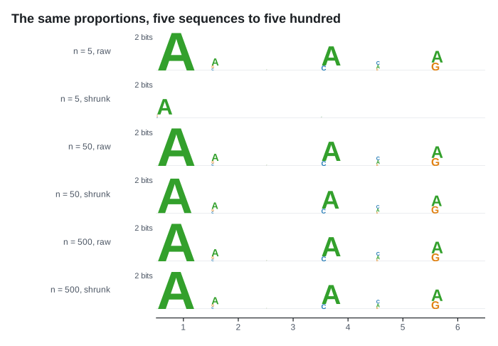
Set alphabet_size(4) for DNA and 20 for protein. Left alone, the alphabet is the set of symbols that appear, which is wrong for a motif where one base never shows up: information content is measured against log2(K), and a uniform background is 1/K.

A logo drawn from four sequences looks identical to one drawn from four thousand. That is an estimation problem, and stabilize() answers it by shrinking each column towards the background by as much as its sample size supports; dash_fit() reports how far each column moved. It needs counts, so a probability matrix also wants sample_size.

Symbols are arbitrary strings, so three letter amino acid codes, codons and k-mers plot as readily as bases:

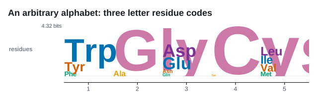
from_sequences upper-cases what it counts and skips - and ., so a column with gaps is normalised over the sequences that have a base there. --logo counts from the first alignment column, so its region is the column range, as in motif:1-8. stacks() returns the computed heights when you want a table rather than a picture.

DynseqTrack¶

Per-base model attribution, drawn as the bases themselves at a height proportional to their score, hanging below the line where the score is negative. A motif the model leaned on reads as a word.

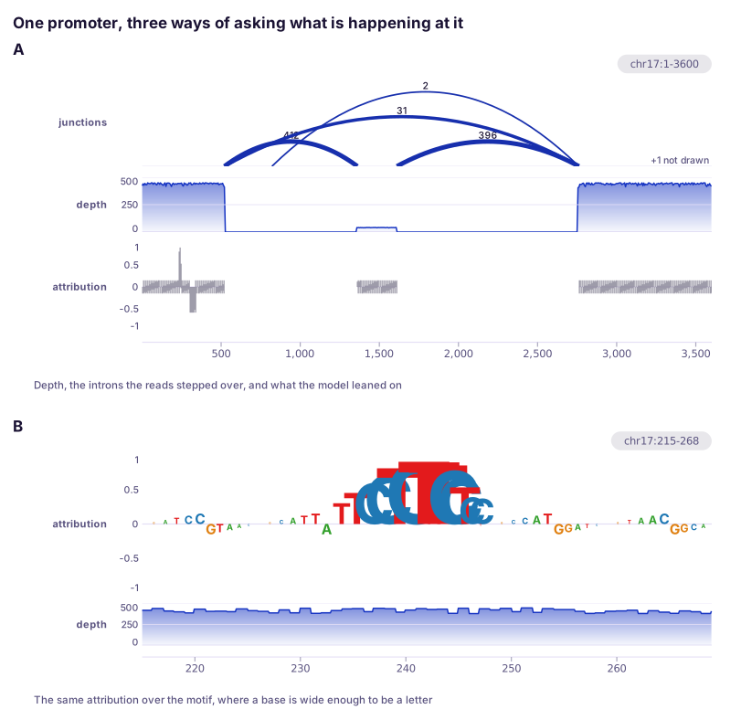
Per-base attribution drawn as letters that stand above or hang below a line, under splice junction arcs and a depth profile, with a close-up where the letters spell the motif


Rust	`.add_dynseq(start, seq, scores)` on `plot()`; `DynseqTrack::new(start, seq, scores)`, `DynseqTrack::from_pairs(start, seq, pairs)`, `DynseqTrack::from_spans(start, seq, spans)`
Command line	`--dynseq FILE --with-sequence FASTA`, with `--height`
Reads	bedGraph of per-base scores (`read::dynseq::scores`), with the letters from the FASTA

RustCommand line

use karyon::plot;

// bases: Vec<u8> and scores: Vec<f64> from 0-based 761,100;
// a score of f64::NAN is a base the model was never run over
plot("NC_000962.3:761,101-761,160")?
    .add_dynseq(761_100, bases, scores)
    .label("contribution")
    .save("attribution.svg")?;

karyon NC_000962.3:761,101-761,160 \
  --dynseq attribution.bedgraph --with-sequence H37Rv.fa --label contribution \
  -o attribution.svg

Options¶

Method	What it does	Default
`.label("contribution")`	Names the track in the left gutter (`--label`)	none
`.height(96.0)`	Band height in pixels (`--height`)	`70`
`.symmetric(false)`	Puts the rule in the middle, reaching equally far either way	on
`.max_extent(1.5)`	Pins how far the axis reaches either side, in the model's units	the largest score in view
`.axis(QuantitativeAxis::new())`	Replaces the value axis	automatic
`.letter_threshold(8.0)`	Pixels a base needs before its letter is drawn	`5`
`.show_scale(false)`	Shows or hides the score axis	shown

Notes¶

The zoom picks one of three regimes: letters where a letter fits, boxes down to a pixel a base, and below that an envelope of the extremes in one neutral ink, never a base colour, because a column spanning forty bases has no base. There is no aggregate to choose: a maximum hides a strong negative, a minimum hides a strong positive, and a mean cancels +2 against -2 into a nought that says the model ignored the place.

A base with no score is not a base scoring nought. The rule is drawn under each run of scored bases rather than across the band, so a stretch the model never saw has no rule under it, while a score of exactly nought sits on one. unscored(&region) counts the bases with a letter and no score.

Two panels of the same height are two different rulers; pin max_extent on both to compare them. --with-sequence is required, because the letters come from it. A FASTA of one record is used whatever its name; of several, the record named like the region's sequence.

Why this is not a logo, or a window track

A LogoTrack normalises within a column, so one symbol carrying one weight takes the whole column whatever the number was: with four bases and one symbol per column, 0.1 and 0.9 both come out at height 1.0 under Probability and both at 8.65 under LogOdds. And LogoColumn::add clamps a negative weight to nought before any score is chosen, so a base the model pulled away from draws as nothing. The magnitude and the sign are the whole measurement.

A WindowTrack also draws a signed statistic against a line, but a window is an interval and a base is not: a megabase of per-base scores would be a million one-base windows. And a base has an identity, which is the letter a reader looking for a motif is reading.