File formats

Which files karyon reads, what it takes from each one, and where each format's coordinates land in the figure.

Nearly every format here is line-based text. The readers live in the library as karyon::read, and each takes a file's text as a string rather than a path, so the same reader serves the command line, the playground and your own program:

use karyon::{plot, read, Region};

fn main() -> Result<(), Box<dyn std::error::Error>> {
    let region = Region::parse("Chr1:1-10,000")?;
    let text = std::fs::read_to_string("genes.bed")?;
    let features = read::interval::features(&text, &region, None)?;

    plot("Chr1:1-10,000")?.add_features(features).save("genes.svg")?;
    Ok(())
}

The karyon command does the same, and adds opening the path. A file compressed with gzip or bgzip is read as the text inside it, and one compressed with bgzip with the .tbi or .csi of tabix beside it is read a window at a time through it, its header and the rows over the window, for the formats whose table below says so. A BAM is read by --coverage, --pileup and --split-reads a window at a time through its .csi or its .bai, as Compressed and binary files shows, and a BCF by --variants, --genotypes and --structural through its .csi, as the VCF it stands for. Three of UCSC's binary formats are read a window at a time through the index each holds: bigWig, bigBed and 2bit, and so is Juicer's .hic, one resolution of it. The readers of all of them take anything that reads and seeks rather than a string. CRAM, and cooler's .cool and .mcool, come in through the tool that writes them as text.

Formats at a glance

Format	What it holds	Read by	Coordinates	Tracks
bedGraph	a value over each interval	--coverage, --windows, --dynseq	0-based, half-open	CoverageTrack, WindowTrack, DynseqTrack
bigWig	a bedGraph's values, indexed, with summaries at coarser scales	--coverage, --windows, --dynseq	0-based, half-open	CoverageTrack, WindowTrack, DynseqTrack
samtools depth	read depth at each position	--coverage	1-based	CoverageTrack
A bare column of values	one value per base	--coverage	none: starts at the region's first base	CoverageTrack
A recombination map	a rate in cM/Mb from each position to the next	--recombination	1-based; a bedGraph of rates 0-based	CoverageTrack
BED	intervals with a name and a strand	--features	0-based, half-open	FeatureTrack
bigBed	a BED's rows, indexed	--features	0-based, half-open	FeatureTrack
GFF3	annotation in nine columns	--features	1-based, inclusive	FeatureTrack
cytoBand	chromosome bands and their stains	--ideogram	0-based, half-open	IdeogramTrack
VCF	small variant calls	--variants	1-based	VariantTrack
VCF with samples	the genotype of each sample at each site	--genotypes	1-based	GenotypeTrack
Structural VCF	structural variant calls	--structural	POS is the base before the event	StructuralTrack
BCF	a VCF's records, binary, indexed	--variants, --genotypes, --structural	0-based, written out 1-based as VCF	VariantTrack, GenotypeTrack, StructuralTrack
Association table	a statistic per tested position	--manhattan	1-based	ManhattanTrack
Matrix table	a value per sample per site	--matrix	1-based, in the header	MatrixTrack
Table of windows	a value per sample per window	--heatmap	0-based, half-open	MatrixTrack
Pairs of positions	a value between two places	--pairs, --ld	PLINK and tables 1-based; BEDPE 0-based, half-open	PairTrack, ManhattanTrack
.hic	a contact map at several resolutions, indexed	--pairs	bins counted from 0, each 0-based and half-open	PairTrack
Selection by site	a test of selection at each site	--selection	sites counted from 1	SelectionTrack
Counts over time	how many of each group at each time, of how many	--frequencies	whole units, as written	SurveillanceTrack
Estimates over time	an estimate at each time, with its interval	--phylodynamics	whole units, as written	PhylodynamicTrack
Segment table	copy number per segment	--copy-number	CNVkit 0-based; ASCAT and .seg 1-based	CopyNumberTrack
FASTA	sequences	--sequence, --orfs, --with-sequence	none: byte n is position n	SequenceTrack, OrfTrack
2bit	sequences, four bases to a byte, indexed	--sequence, --orfs, --with-sequence	none: base n is position n	SequenceTrack, OrfTrack
Aligned FASTA	an alignment	--msa, --snps, --logo	alignment columns	MsaTrack, SnpTrack, LogoTrack
Newick	a phylogeny	--tree, --tanglegram, --against, --with-tree	none	TreeTrack, TanglegramTrack, CladeTrack
SAM	aligned reads	--pileup	1-based	PileupTrack
SAM with SA tags	reads aligned in pieces	--split-reads	1-based	SplitReadTrack
SJ.out.tab	splice junctions	--junctions	1-based, inclusive, on the intron	JunctionTrack
bedMethyl	modified bases per strand	--methylation	0-based, half-open	MethylationTrack
Bismark extractor file	methylation calls per read	--bisulfite	1-based	BisulfiteTrack
SLOW5	the raw current of nanopore reads	--squiggle	samples counted from 1	SquiggleTrack
PAF	alignments between two sequences	--synteny, --dotplot	0-based, half-open	SyntenyTrack, DotplotTrack
Gene neighbourhoods	BED or GFF3 with a genome per row	--loci	as BED or GFF3	LocusTrack
Homology table	which genes match which	--links	none	LocusTrack
InterProScan table	protein domains	--domains	1-based, inclusive, in residues	DomainTrack
Gubbins clade blocks	spans carried by named taxa	--clades	1-based, inclusive	CladeTrack
Sample sheet	what is known about named rows	--traits	none	strips beside a track's rows

The region you type is always 1-based and inclusive, as samtools and IGV write it, whatever the files use: chr1:101-200 is the bases numbered 100 to 199 from zero. Every reader converts its own format on the way in, so all of them land in the same place. Coordinates has the whole convention.

How a file is read

Each flag reads one format, so most files are never guessed at. Three flags accept more than one and tell them apart by looking, as the next section explains.

Skipped or refused

A row on another sequence, or outside the window, is skipped without a word. Handing over a whole genome and drawing one window of it is the normal way to use a reader.

A row that does not parse is never skipped. It stops the figure and names the line:

karyon: --coverage depth.txt: line 3: depth is not a number: "NA"

Before a reader looks at a line, these are dropped: blank lines; lines starting with # (comments, GFF3 pragmas, the VCF header) or @ (the SAM header); a UCSC track or browser line, but only one carrying a key=value, since a sequence may be called track; a byte order mark at the start of the file; and the carriage return of a Windows line ending. A Newick file is the exception: it is read whole, as one tree, though its byte order mark is dropped all the same.

Fields are split on tabs when a line holds a tab, and on runs of spaces when it does not, so tab-separated and space-separated files read the same. A field that holds a space, or an empty field, needs a tab-separated file, since runs of spaces collapse into one separator. The InterProScan table must be tab separated.

The line number in a message counts the dropped lines, so it is the line number in your editor. Most readers check a row's shape before its sequence name, so a malformed row anywhere in the file stops the read; the BED, GFF3 and cytoBand readers compare the name first, so a broken row on another chromosome goes past unread.

In the tables below, Skipped lists what a reader passes over besides rows on another sequence and rows outside the window, and says so where a format has no sequence to compare. Refused lists what stops the read besides a number that does not parse, which every reader refuses except where a section says otherwise.

Why a broken row stops the figure rather than being skipped

A row on another sequence was never part of the figure. A row that does not parse says the file is not what the flag claimed, and reading past it would draw a figure with data missing and nothing on it to say so. That is worse than no figure, so the read stops on the line.

How long a sequence is

A sequence named as the place is drawn whole, as long as one of the figure's files says it is: a FASTA record's length; a BAM's header, or a SAM's @SQ LN; a VCF's or BCF's ##contig=<ID=NC_000962.3,length=4411532>; a GFF3's ##sequence-region NC_000962.3 1 4411532 among its opening lines; the index of a bigWig, a bigBed or a 2bit; a .hic's header; or a PAF's query length. With none of them a figure along the sequence ends where its rows reach, and says so. A circle, --circular, is refused instead, since it closes where the sequence ends and a ring closed early puts every position round it at the wrong angle; write the span from base 1, as NC_000962.3:1-4,411,532, to give the length yourself. Where two files give different lengths, a figure along the sequence takes the first one's, and a circle is refused, naming each file and the length it says.

Telling formats apart

A coverage file

--coverage accepts three shapes, and the column count is the only difference between them:

Columns	Read as	Example line
4	bedGraph	chr2L 100 103 5
3	samtools depth	chr2L 100 5
1	a bare column of values	5

The shape is decided on the first data line, and a file whose column count changes partway is refused on the line where it changed. --format bedgraph, --format depth or --format values decides instead. --format bed and --format gff3 are refused here, because those formats name intervals rather than a value per base.

samtools depth over more than one file

samtools depth a.bam b.bam writes one depth column per file, so two files make four columns, the shape of a bedGraph. Read that way, the position becomes a start, the first depth an end and the second depth the value: a plausible figure of nothing.

karyon catches it. A depth is nearly always smaller than its position, so the first record ends before it starts, and depth records overlap where bedGraph intervals never do. Either is refused with the way out:

karyon: --coverage depth.txt: line 1: end is before start, so this is not a bedGraph. samtools depth over more than one file also writes four columns, and its second column is a position rather than an end: pass --format depth to read it as that, or --format bedgraph to insist

--format depth reads the first sample and ignores the other depth columns. --format bedgraph insists on bedGraph, which is also how to read a bedGraph whose rows are out of order.

A three-column BED is read as depth

A BED with three columns has no value column whose absence could be noticed, so --coverage reads chr1 100 200 as position 100 with a depth of 200, and nothing warns. A BED belongs to --features. To draw intervals as a signal, give each a value in a fourth column and read it as bedGraph.

A feature file

--features and --loci read BED or GFF3, GTF counting as GFF3, and decide which in this order:

1. --format bed or --format gff3, if given.
2. A ##gff-version line anywhere in the file means GFF3.
3. Column seven of the first data row: GFF3 puts the strand there, so +, -, . or ? means GFF3. A BED of nine or more columns puts thickStart there, a number.
4. Anything else, including a first row shorter than seven columns, is BED.

Reading one format as the other moves every feature by a base without failing, which is why the order is fixed and --format can overrule it.

The words --format takes

Word	Reads as	Used by
bedgraph, bg	bedGraph	--coverage
depth	samtools depth	--coverage
values	a bare column of values	--coverage
bed	BED	--features, --loci
gff3, gff, gtf	GFF3	--features, --loci

--format is refused after the tracks that read a single format, and so is a word the track before it does not read: a signal word after --features would change nothing, since the guess runs as usual.

gtf is a spelling of gff3, not a GTF reader

A GTF's first eight columns are GFF3's, so its coordinates come out right, and its seventh column is a strand, so it is read as GFF3 even without --format. Its ninth column is gene_id "..."; gene_name "..."; rather than key=value, so no name is found and the features are drawn unnamed.

Signal

bedGraph

A value over each interval: a depth, a score, a statistic.

track type=bedGraph name=coverage
chr2L  100  103  5
chr2L  103  105  9

Read by	--coverage, --windows and --dynseq; read::signal::spans, read::signal::windows and read::dynseq::scores, and read::signal::genome_spans and read::signal::genome_windows for every sequence
Columns	1 sequence, 2 start, 3 end, 4 value
Coordinates	0-based and half-open, passed through: 100 103 is the bases 100, 101 and 102, and 103 belongs to the next row
With an index	read a window at a time, through the .tbi that tabix -p bed depth.bedgraph.gz writes or the .csi mosdepth writes, as the guide says; a track line has to be skipped as well, with -S1
Refused	an end before its start

The three flags read it differently:

	--coverage	--windows	--dynseq
Columns	exactly four	four or more, the rest ignored	four or more, the rest ignored
A row becomes	its value on every base it covers	one window, kept whole	its score on every base it covers
A base no row covers	0	nothing drawn	unscored: no letter, and a gap in the rule beneath
A value that is not a number	refused, but nan and inf are read as missing and leave a gap	refused, but nan and inf leave their window empty	leaves its bases unscored

--coverage also refuses overlapping rows, the sign of two-sample depth, unless --format bedgraph is given.

Named with no place, after --coverage or --windows or on its own, a bedGraph is read whole and drawn across the whole genome: every sequence it names, end to end, in the order chromosomes are counted, each as long as its furthest row reaches or another file of the figure reaches further. Rows overlap only on one sequence, so the first row of the next sequence starting back at 0 is no overlap. A base no row covers on a sequence the file names is still 0, and a sequence it names no row on, which another file of the figure does, is no value at all, a gap in the profile: a file that left a chromosome out has said nothing about it. mosdepth's .regions.bed.gz, the depth in the windows mosdepth --by counts, is a bedGraph by another name and is drawn the same way.

bigWig

A bedGraph's values, or a wiggle file's, packed into blocks behind an index, with the same values summed up again at a few coarser scales, the zoom levels. UCSC's bedGraphToBigWig and wigToBigWig write it, and so does deepTools' bamCoverage.

Read by	--coverage, --windows and --dynseq, or a .bw or .bigwig named on its own; read::bigwig::window, and read::bigwig::genome for every sequence
What is read	the blocks over the window, through the index: its bedGraph, variable-step and fixed-step sections alike, as bigWigToBedGraph prints them
Coordinates	0-based and half-open, as bedGraph, passed through
A base no value covers	0, as in a bedGraph
Refused	a place on a sequence the file does not name, with the ones it does, where it is the figure's one place; a file damaged or cut short; the file compressed with gzip, with the gunzip -k that gives it back; --format, since the file says what it holds; the file on standard input, since it is read out of order

kent indexes only the sequences that hold data, so a bigWig written against a genome's lengths names those and no others. Over several places, one on a sequence it does not name holds none of its values and says so there, as the bedGraph it was written from does.

--coverage reads it at the scale it is drawn at. Where a pixel holds two bins or more of a zoom level, the coarsest such level is read instead of the values as written, and each bin is painted over its bases with what --aggregate takes of a pixel: its highest value, its lowest, or its sum spread over its bases, with the bases no value covers counted as 0 in each. A chromosome of 249 Mb written as 4.7 million spans, a 38 MB bigWig, is then 5,139 bins of 51,200 bases, and draws 900 pixels wide in 0.01 s and 4 MB, where its bedGraph takes 0.95 s and 216 MB. The figure is the one the values as written draw, but for a bin that straddles two columns and lends its highest value to both, so a peak may be drawn a column wider than it is, as in UCSC's browser: over that chromosome 154 of 792 columns came out higher and none lower. The scale is theirs too, up to the highest value under the window, whether the bins are drawn by their highest value, their lowest or their mean. A window of 10 kb of it reads 189 spans as written and draws byte for byte what the bedGraph draws. A file written without zoom levels is read as written at any scale. --windows and --dynseq always read the values as written.

With no place, --coverage draws a bigWig across the whole genome, each sequence it names as long as its index says, read from the zoom level of which a pixel of the whole genome holds two bins, as a window is: a genome of three billion bases 900 pixels wide is a few thousand bins of the summary the file keeps at that scale. --windows reads it whole, as written. After --dynseq a bigWig still needs a place, since its scores are drawn as the bases under them.

samtools depth

The read depth at each position, as samtools depth writes it.

# samtools depth -a -r NC_000962.3:761100-761102 aln.bam
NC_000962.3  761100  12
NC_000962.3  761101  14
NC_000962.3  761102  0

Read by	--coverage, with a place or across the whole genome as bedGraph is; read::signal::spans and read::signal::genome_spans
Columns	1 sequence, 2 position, 3 depth; with --format depth, further depth columns are ignored
Coordinates	1-based: position 761100 is 0-based 761099
With an index	read a window at a time, through the .tbi that tabix -s1 -b2 -e2 depth.txt.gz writes
Refused	a position of 0

Without -a, samtools leaves out positions no read covers. Those stay at 0 anyway, so the figure is the same.

A bare column of values

One number per line, for anything already computed base by base.

0.5
0.25
0.75

Read by	--coverage; read::signal::spans
Columns	1 value
Coordinates	none: the first value is the region's first base, the next value the base after it
Skipped	values past the end of the region; the file names no sequence
Refused	with no place, since there is no sequence to lay the values on

The file carries no position, so it belongs to one window: drawn over chr4:501-600 and over chr4:1-100, the same file puts its values in two different places. If it runs out before the region does, the rest stays at 0.

A recombination map

The rate of recombination along a chromosome, as HapMap writes a genetic map: a rate in centimorgans per megabase at each position, holding to the next.

Chromosome  Position(bp)  Rate(cM/Mb)  Map(cM)
chr1        604401        0.84         0.000000
chr1        609401        0.63         0.004200

Read by	--recombination, or a file whose name holds genetic_map, as a track of its own; --with-recombination after --manhattan, laid over the scan; read::recombination::rates
Columns	found by name in any case: a position (Position(bp), position), a rate (Rate(cM/Mb), COMBINED_rate(cM/Mb)) and, where there is one, a chromosome; with no header, a bedGraph of rates
Coordinates	positions 1-based; a bedGraph 0-based, half-open
With an index	read whole all the same: each rate runs on to the next row, so the rows either side of a window belong to it, and 290 windows of 300 drew differently from their rows alone
Skipped	rows on another sequence; a rate that is empty or NA, which leaves its stretch out rather than at nought
Refused	a position of 0; a negative rate

The maps that come with IMPUTE2 and SHAPEIT are one chromosome to a file, with no chromosome column, position COMBINED_rate(cM/Mb) Genetic_Map(cM), and read the same. The rows are put in order first, and the last position's rate covers that one base. The track is a line in cM/Mb, the highest rate in each pixel, so a hotspot narrower than a pixel is still drawn.

Intervals

BED

Intervals with a name and a strand.

track name=genes description="TAIR10"
Chr1  3630  5899  AT1G01010  0  +
Chr1  6787  9130  AT1G01020  0  -
Chr2  3000  4000  AT2G01010  0  +

Read by	--features; read::interval::features. --loci reads it as gene neighbourhoods, and --codons reads its thick span, cut by its blocks, as the CDS
Columns	1 sequence, 2 start, 3 end, 4 name (. for none), 6 strand (+ or -; anything else is unknown); 7 and 8, thickStart and thickEnd, the part that codes, and 10 to 12 the blocks of a BED12, which are its exons
Ignored	5 score and 9 colour; column 7 also tells a BED from a GFF3
Coordinates	0-based and half-open, passed through: 3630 5899 is the bases 3,631 to 5,899 counted from 1
With an index	read a window at a time, through the .tbi that tabix -p bed genes.bed.gz writes
Refused	fewer than 3 columns; an end before its start

Over Chr1:1-10,000 this file draws the two Chr1 genes and skips the Chr2 row; the track line is dropped because it carries key=value pairs.

bigBed

A BED's rows packed into blocks behind an index, as UCSC's bedToBigBed writes them, with an autoSql description of any columns of its own.

Read by	--features, or a .bb or .bigbed named on its own; read::bigbed::bed, which writes the rows over a window back out as BED for read::interval::features
Columns	the ones the header says are BED's own (definedFieldCount), and none after: all twelve of a BED12, so a gene keeps its exons and the stretch that codes; six of a narrowPeak, which is BED6 and four columns of its own
Coordinates	0-based and half-open, as BED, passed through
Refused	a place on a sequence the file does not name, with the ones it does, where it is the figure's one place; a file damaged or cut short; the file compressed with gzip, with the gunzip -k that gives it back; --format; the file on standard input

The columns past BED's own are left out because they are the file's own: a narrowPeak's seventh is a signal value, and read as BED it would be a BED12's thickStart, a coding stretch starting at 5.2. A row that starts before the window and runs into it is kept whole, as in a BED.

A gene a bigBed names is a place a figure can be drawn over, as karyon geneA genes.bb, and so is a --shade by its name. The window is read through the index, but a name is found by reading every row, so a bigBed larger than 64 MB is not read for one; the figure says so, and its place is written as a span instead. Each row's sequence is looked up by its number, so a file of many sequences costs no more: placed by a name in one of 20.9 MB naming 200,000 sequences, a figure is drawn in 0.9 s, where it took 16 s.

Like a bigWig, a bigBed names only the sequences that hold rows, and over several places, one on a sequence it does not name says it has no features there, as the BED it was written from does.

GFF3

Annotation in nine columns.

##gff-version 3
#!genome-build H37Rv
NC_000962.3  RefSeq  gene  759807  763325  .  +  .  ID=gene-Rv0667;Name=rpoB
NC_000962.3  RefSeq  gene  763370  767320  .  +  .  ID=gene-Rv0668;Name=rpoC

Read by	--features; read::interval::features. --loci reads it as gene neighbourhoods, --clades as clade blocks
Columns	1 sequence, 3 type, 4 start, 5 end, 7 strand, 9 attributes: the name is Name=, failing that gene=, failing that ID=
Ignored	2 source, 6 score, 8 phase
Coordinates	1-based and inclusive: the start moves back one and the end stays, so 759807 763325 is 0-based 759806..763325
With an index	read a window at a time where its first line is ##gff-version 3, through the .tbi that tabix -p gff genes.gff3.gz writes once the file is sorted with sort -k1,1 -k4,4n; read over the window, then over as far as the genes over it reach, so a gene whose intron covers the window keeps every exon. A GTF is read whole: UCSC's has no gene or transcript rows, and a window inside an intron holds no row of its gene. So is a GFF3 whose exons name a transcript it has no row for, which the rows it opens with or the rows over the window show
Skipped	a trailing ##FASTA section, whose lines name no sequence; a row describing the whole sequence; a row whose parent is in the file
Refused	fewer than 5 columns; a start of 0; an end before its start

Attribute values are percent-decoded, so Name=chromosomal%20replication%2C%20initiator reads as chromosomal replication, initiator.

--features draws each thing once. An annotation writes a gene at every level, the gene, its transcripts, their exons and the CDS, and a row whose Parent= or Derives_from= names a row in the file is left out, so the gene stands for all of them. A part whose whole is not in the file, a file cut down to CDS rows for instance, is drawn. A region, chromosome, scaffold, supercontig, databank_entry or source row that starts at base 1 describes the sequence rather than something on it, as NCBI's first row for each sequence does, and is left out too. To draw one level on purpose, filter first:

awk '$3 == "CDS"' annotation.gff3 \
  | karyon NC_000962.3:759,000-768,000 --features - --label CDS -o cds.svg

GTF is read as GFF3 is, with its key "value"; attributes: a gene is named by gene_name and failing that gene_id, a transcript by transcript_name or transcript_id, and anything else by the gene it belongs to. A transcript stands for its exons and a gene for its transcripts in the same way, so GENCODE draws one row a gene, StringTie, which writes no gene rows, one a transcript, and a table browser GTF of exons alone one an exon.

--codons reads the same rows for what codes (read::interval::coding): each transcript's CDS rows, with a GTF's stop_codon where it lies past them, cut by its exons, and a CDS row under no gene as a coding sequence of its own, with every other row under its ID=. The rows are kept apart, each with its phase, column 8, so two that share a base, as NCBI writes a ribosomal slippage, are a change of frame and not one stretch, and a 5'-most row of phase 1 or 2, or one NCBI marks with start_range (end_range on the reverse strand), is a CDS that does not begin on its start codon. A gene row alone says where a gene is and not where its CDS starts, so a file without CDS rows draws no codon ruler. The transl_table= a CDS row carries, as NCBI writes one, is the translation table its codons are read with, and --genetic-code overrules it (read::interval::translation_table).

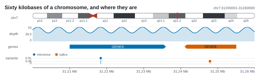
cytoBand

Chromosome bands and their Giemsa stains, as UCSC distributes them.

chr21  0         2800000   p13    gvar
chr21  2800000   6800000   p12    stalk
chr21  6800000   10900000  p11.2  gvar
chr21  10900000  13200000  p11.1  acen
chr20  0         5100000   p13    gneg

Read by	--ideogram; read::interval::cytoband
Columns	1 sequence, 2 start, 3 end, 4 band name, 5 stain; only the first three are required
Coordinates	0-based and half-open, passed through
Skipped	rows on another sequence only: the window does not filter this file
Refused	on the region's sequence, fewer than 3 columns or an end before its start

The ideogram draws the whole chromosome and marks the window on it, so every band on the region's sequence is kept, and the chromosome's length is the highest end among them. The stains are the UCSC words, in any case: gneg, gpos25, gpos50, gpos75, gpos or gpos100, acen, gvar and stalk. A missing or unknown stain is drawn as the palest band rather than guessed at.

Calls and statistics

VCF

Small variant calls.

##fileformat=VCFv4.2
#CHROM       POS    ID  REF   ALT  QUAL  FILTER  INFO
NC_045512.2  21563  .   A     G    900   PASS    DP=54;AF=0.98;ANN=G|missense_variant|MODERATE|S
NC_045512.2  21990  .   TTTA  T    500   PASS    DP=40

Read by	--variants; read::point::variants
Columns	1 CHROM, 2 POS, 4 REF, 5 ALT (one call per alternate allele), 8 INFO: AF, ANN, BCSQ
Ignored	3 ID, 6 QUAL, 7 FILTER, and 9 onwards, which --genotypes reads, so a call that failed a filter is still drawn and a sites-only VCF reads like a cohort's
Coordinates	1-based: POS 21563 is 0-based 21562
With an index	read a window at a time, through the .tbi that tabix -p vcf calls.vcf.gz writes or the .csi of bcftools index; the header comes with every window. The same calls as BCF are read through theirs and draw the same figure
Skipped	a gVCF's reference blocks, rows whose ALT is . or only a placeholder, <NON_REF> as GATK writes one and <*> as bcftools does; and the placeholder of a variant row written T,<NON_REF>, which draws its T alone
Missing	an AF of ., the missing value bcftools writes for a fraction it could not work out, is no fraction, for the row as AF=. or for one allele as AF=0.5,.
Refused	fewer than 8 columns; a POS of 0; an AF whose count is neither 1 nor the number of alternate alleles

• Height is the allele fraction, AF, matched as a whole key so that MLEAF and AF_ESP are not taken for it. One number on a multi-allelic row is shared, and a row with none, or an allele whose AF is ., is drawn at 1.0: a call with no fraction is still a call.
• Category is what an annotator wrote: the ANN entry naming this allele (from snpEff or VEP), or else the first; or the first BCSQ consequence (from bcftools csq), without the * of an uncertain one. With neither, it is the shape of REF against ALT: substitution, insertion or deletion by length, breakend for square brackets, and deletion for *. A symbolic allele is named by its tag: <DEL> is deletion, <INS:ME:ALU> is insertion, and <DUP> is dup.
• Reach: a call is kept when what REF spells touches the window, not only its first base, since a deletion is written one base to the left of what it removes.

VCF genotypes

The genotype of each sample at each site of a cohort, as a joint caller or bcftools merge writes it: the eight columns of a site, then the keys of the sample columns, then a column per sample.

#CHROM       POS     ID   REF  ALT  QUAL  FILTER  INFO  FORMAT  S01  S02    S03
NC_000962.3  761155  .    C    T    60    PASS    .     GT:DP   0:31 1:28   .
NC_000962.3  762368  rs1  G    A,T  60    PASS    .     DP:GT   30:1 29:2   31:0

Read by	--genotypes; read::point::genotypes, and read::point::samples for the names alone
Columns	1 CHROM, 2 POS, 3 ID, 4 REF, 5 ALT, 9 FORMAT (GT found among its keys by name, wherever it is), and 10 onwards, one sample each, named on the #CHROM line in the same order
Ignored	6 QUAL, 7 FILTER, 8 INFO, and every key of FORMAT but GT
Coordinates	1-based: POS 761155 is 0-based 761154, the base the record's lollipop stands on
With an index	read a window at a time, as a VCF is: the #CHROM line that names the samples comes with every window
Skipped	rows on another sequence, rows whose REF does not reach the window, and a gVCF's reference blocks, rows whose ALT is . or only <NON_REF> or <*>
Not called	., ./., an empty field, a sample field cut short before its GT, a call with any copy unknown, as ./1, and every sample of a row whose FORMAT has no GT
Refused	no #CHROM line, which bcftools view -H leaves out; a #CHROM line naming no sample, or one sample twice; a row with more or fewer samples than it names; a GT that is not allele numbers and dots; an allele number past the row's alternates; and a window whose rows none of them carries GT

• GT is allele numbers joined by /, or by | where the call is phased, with the leading / or | that VCF 4.4 allows: 0 is REF and i is the ith allele of ALT. One number is a haploid call, two a diploid one and more a polyploid one, read up to 255 copies.
• What is drawn is the share of the copies that are not REF: 1 and 1/1 all of them, 0/1 half and 0/0/0/1 a quarter. 1/2 has no copy of REF and is all alternate, and so is a copy that names *, the base a deletion upstream took away, or a placeholder, <NON_REF> or <*>, which says the base is not REF without saying what it is: any number but 0 is an alternate copy.
• A polyploid call keeps the alleles of its first two copies and the count of its alternate copies, so its tooltip spells out two alleles and says how many more copies there are and how many of all of them are alternate.
• Reach: a row is kept by the rule a VCF row is, when what REF spells touches the window. A row outside the window is not split past its position, so a cohort of a thousand samples costs little for the rows a figure does not draw. With its .tbi or .csi beside it, the rows a figure does not draw are not read at all: a window of 2,000 bases of 200 samples' calls, 825 MB of text, takes 8 ms where it took 2.8 seconds.

Structural VCF

Structural calls, drawn as arcs between their breakpoints.

#CHROM  POS     ID     REF  ALT             QUAL  FILTER  INFO
chrA    321682  del_1  T    <DEL>           6     PASS    SVTYPE=DEL;SVLEN=205;END=321887
chrA    321687  bnd_W  T    T[chrA:323457[  6     PASS    SVTYPE=BND;MATEID=bnd_Y

Read by	--structural; read::structural::variants
Columns	1 CHROM, 2 POS, 3 ID (the call's name), 4 REF, 5 ALT, 8 INFO: SVTYPE, SVLEN, END, and read support from the first of SUPPORT, PE, SR, RE and DV
Ignored	6 QUAL, 7 FILTER, 9 onwards
Coordinates	POS is the base before the event and END its last base, so both pass through unchanged: the deletion above covers 321,683 to 321,887 counted from 1
With an index	read whole all the same: an arc is drawn from the lower of its two breakends, which lies outside a window the arc crosses
Skipped	rows with no symbolic allele and no SVTYPE; classes with no glyph, such as <CNV>; a breakend whose mate is on another sequence, and a single breakend; the second record of a breakend pair
Missing	an SVLEN or END of ., the missing value, is no length, as a key that is not there is none
Refused	fewer than 8 columns; an SVLEN and END that disagree; a symbolic call with neither; a call that covers no bases; an end before its start

This is the one VCF reader that takes nothing off POS: a symbolic allele cannot be written without a reference base, so the specification puts POS on the base before the event. The class comes from ALT (square brackets for a breakend, then <DEL>, <DUP>, <INV>, <INS>), or else from SVTYPE (DEL, DUP, INV, INS, BND, TRA). The length comes from SVLEN, taken as a positive number since VCF 4.3 writes a deletion's as negative; failing that from END; and for a call spelled out in full, from the length of REF. An insertion has one breakpoint and no footprint. A breakend pair is one arc: the mate is read from the ALT itself, and only the record at the lower position draws it.

BCF

A VCF's records in binary, as bcftools view -Ob writes them: each number stored as a number, and each name a VCF spells out on every row, a sequence, a filter, an INFO or a FORMAT key, stored as its place in a dictionary the header keeps. It is BGZF, as a bgzipped VCF is, and bcftools index writes the .csi beside it.

Read by	--variants, --genotypes and --structural, or a .bcf named on its own, as its calls; read::bcf::window
What is read	the header, and the records over the window, written as the VCF text bcftools view prints for them, byte for byte, which the VCF, VCF genotypes and structural VCF readers then read
Of each sample	nothing for --variants and --structural, whose records' samples' columns are passed by undecoded, as bcftools view -G prints them; GT alone for --genotypes
Coordinates	stored 0-based, written out 1-based as VCF: a record stored at 99 is written at 100, and read at 99
With an index	read a window at a time through the .csi beside it, calls.bcf.csi or calls.csi: only the blocks that hold records over the window. Without one, every record is read and those over the window kept, since a file with no index need not be sorted. Structural calls are read whole either way
Not trusted	a .csi older than its file, one that does not read as an index, and one whose first record is not where the file's header ends, as the index of another file: the file is read whole, which draws the same figure, and a note says why
Refused	a file of another version than 2.2, which is all htslib reads; a record whose parts do not fit the bytes it says it holds; a value of a type BCF does not have; a sequence or a key the header does not name; a record of more or fewer samples than the header names; the file on standard input, since it is read from its bytes, where the text bcftools view writes is what a pipe takes; --format

A record is over the window where the bases it spans touch it: from its position as far as its reference allele spells or as its END says, whichever is further, which keeps every record the readers of VCF keep, and they drop the rest by their own rule, as they drop a VCF's rows outside the window. A record a reader refuses is named by its place, as the record at chr1:60,000, since a BCF has no line to number.

A float is written as htslib writes it, six significant digits rounded its own way, so a value is the number bcftools view prints for it: AF stored as 0.3333333 is drawn at 0.333333, as bcftools prints it. Under VCF 4.4 a GT keeps the / or | before its first allele that bcftools prints.

The association table

A statistic per tested position, for a Manhattan plot.

chrom         pos   neglog10p
Pf3D7_07_v3   4100  8.49
Pf3D7_08_v3   4110  12.0
Pf3D7_07_v3   4150  0.40

Read by	--manhattan; read::point::associations
Columns	two or three: an optional sequence name, then a position and a value; or an association tool's own table, read by its header
Coordinates	1-based: position 4100 is 0-based 4099
With an index	read a window at a time over a place: through the .tbi that tabix -s1 -b2 -e2 scan.tsv.gz writes for PLINK 2's #CHROM line or a table of three columns, and -S1 with the table's own columns for a plain header, as -S1 -s1 -b3 -e3 for PLINK 1 once its columns, padded with spaces, are turned into tabs, as the guide shows. A table with no header whose values over the window all lie between 0 and 1 is read whole, since every value it holds says whether they are p-values
Skipped	a header on the first line; a two-column table names no sequence; in a tool's table, a test written NA
Refused	in a table of two or three columns, a line of any other number; a tool's table whose header names no position or no p-value; a position of 0; a header-like word after the first line; in a column of p-values, a value outside 0 to 1; with no header, a file whose every value lies between 0 and 1

A scan is drawn higher meaning stronger, and the header says what the value column holds:

• p-values: a column named P, pvalue, pval, p.value, P-value, or starting with p_ as p_wald and P_BOLT_LMM do, and a q-value, FDR or padj column, is drawn as -log10 of itself, and the axis says -log10 p. --threshold is then a p-value too: --threshold 5e-8 draws the line where genome-wide does.
• Anything else is drawn as written, in the units --threshold is given in. A name that mentions a logarithm, as LOG10P, -log10(p) and mlog10p do, is always read as one already taken.

A table with no header says nothing about its values. If every one of them lies between 0 and 1 it is refused, since that is how p-values look and drawn as written they put the strongest hit at the bottom; add a first line naming the column, P to have the values converted or what they are to have them drawn as written.

An association tool's own table, wider than three columns, is given as it is and read by its header. The position is the column named BP, POS, GENPOS, PS or base_pair_location; the sequence, when there is one, CHR, CHROM, #CHROM, chromosome, seqname or contig; and the value the p-value column, or failing one the column naming its logarithm, as LOG10P does. That is what PLINK, PLINK 2, REGENIE, BOLT-LMM, GEMMA, SAIGE and the GWAS Catalog write. A test the tool could not run is written NA and left out, and a header that names no position or no p-value is refused with the names it does give. The tools write a chromosome as a number, 1 where a FASTA may say NC_000962.3; --rename 1=NC_000962.3 reads the table by the FASTA's name, and a figure on a name the table does not use says which --rename would draw it:

karyon 7:1-159,345,973 --manhattan scan.assoc --threshold 5e-8 -o scan.svg

The matrix table

A value per sample per site: an allele fraction, a genotype, a depth.

sample   14150  14180  14212
BY4741   1      0      .
RM11-1a  1      1      NA
YJM789   0      0      1

Read by	--matrix; read::table::matrix
Columns	a header of site positions, then one row per sample: its name and one value per site
Coordinates	1-based positions in the header: 14150 is 0-based 14149
Skipped	sites outside the window, each taking its column out of every row; the table names no sequence
Refused	a header position of 0; a row whose count of values differs from the header's count of sites

The first header field is the table's corner: a word such as sample, or empty in a tab-separated file. An empty cell, . and NA are missing, drawn as a hole rather than as the bottom of the colour ramp; a typed 0 is a value, and any other word is refused.

The table of windows

A value per sample per window: a depth, a copy number, a methylation level, as bedtools unionbedg -header writes it.

chrom        start   end     S01    S02    S03
NC_000962.3  0       100000  68.1   103.2  54.9
NC_000962.3  100000  200000  70.4   98.7   0.0

Read by	--heatmap; read::table::windows
Columns	a sequence, a start and an end, then one value per sample; the header names the samples
Coordinates	0-based, half-open, as BED; passed through
With an index	read a window at a time, through the .tbi that tabix -s1 -b2 -e3 -0 -S1 windows.tsv.gz writes for a table with its header on the first line; a long table is read whole, since it names its samples on its rows
Skipped	windows on another sequence or outside the region, and a window that ends where it starts
Refused	a line after the header that is not a window; a window whose count of values differs from the count of samples

deepTools' multiBigwigSummary --outRawCounts writes the same shape under a header of its own, #'chr' 'start' 'end' 'S01.bam', which is read with its hash and quotes taken off. A table with no header names its samples by their column, column 4 onwards. An empty cell, . and NA are missing, as in the matrix table. --relative divides each sample by its own median over the windows drawn, so 1× is its usual value, and reads it either side of 1×, a loss in one hue and a gain in the other; --center reads the values either side of a value of its own, as --center 0 for a log ratio.

The long form, one sample of one window to a row, is read too: a sequence, a start and an end, then the sample and its value.

chrom        start   end     sample  depth
NC_000962.3  0       100000  S01     68.1
NC_000962.3  0       100000  S02     103.2

It is told from the wide table by its fourth column, which names a sample: the header calls it sample, name or id, or the first window holds a word there. A sample with no row in a window is missing there. Two values for one sample in one window, and two windows that overlap without being the same window, are refused.

Pairs of positions

A value between two places: the linkage between two variants, the contacts between two bins, a score between two sites. Three shapes, told apart by the first line.

PLINK's .ld table, as --r2 writes it, its columns found by their names:

 CHR_A    BP_A   SNP_A  CHR_B    BP_B   SNP_B      R2
     1  754400  rs101      1  756600  rs102   0.8412

BEDPE, two stretches and a value, as cooler dump --join writes a contact map and loop callers write their loops:

chr2  0      10000  chr2  20000  30000  57

A table of your own, headed by what its columns are:

pos1     pos2     score
761110   761155   0.82

Read by	--pairs, and --ld after --manhattan; read::pairs::pairs
Columns	PLINK: BP_A and BP_B, the value as R2, R or DP, the sequences as CHR_A and CHR_B. BEDPE: chrom1 start1 end1 chrom2 start2 end2, and the first number after them as the value, 1 where there is none. A table: two positions (pos1 and pos2, site_a and site_b, bp_a and bp_b), a value (r2, score, count, weight, value) and a sequence (chrom) where there is one; three columns with no header are two positions and a value
Coordinates	PLINK and a table: 1-based. BEDPE: 0-based, half-open
Skipped	a pair with either place on another sequence
Refused	a header with no two columns of positions; a position of 0; a BEDPE row of fewer than six columns

Tabs, commas or runs of spaces separate the columns. An empty value, ., NA or nan is a pair with no answer, kept and not drawn. A value named as a correlation, R2, r², R or D', is keyed from 0 to 1 whatever the strongest pair in the window, and drawn as a triangle.

A contact map in Juicer's .hic is read as it is, as the next section says. One in cooler's .cool or .mcool is not, and is answered with how to write it as the BEDPE above. A .cool is one command, --pairs <(cooler dump --join -r REGION contacts.cool). A .mcool holds several resolutions, which cooler ls lists, and one is written as contacts.mcool::/resolutions/10000; hictk dump --join --resolution 10000 -r REGION contacts.mcool writes the same rows. Both are HDF5, a file system in a file: a superblock, object headers, B-trees, heaps and datasets in chunks through filters, each in more than one version, and h5py, which cooler writes through, writes either of two families of them by the library version it is told to keep to. Reading them is a reader of HDF5 of its own, which the crate's promise of no dependencies leaves to be written by hand, and reading one family alone would make a file read or not by how its writer was set up, so a cooler file comes in through the tool that writes its text.

.hic

A Hi-C contact map as Juicer's tools and hictk write it: for each two sequences and each size of bin, how many read pairs joined each two bins, kept in blocks compressed with zlib behind an index, several resolutions in one file. hictk load writes one from text, and hictk zoomify adds the coarser resolutions.

Read by	--pairs, or a .hic named on its own; read::hic::contacts, which hands the cells over as pairs, written out for the reader of pairs as the BEDPE hictk dump --join prints, cell for cell, which a test holds it to
What is read	the header, the master index at the end of the file, the list of blocks of the map of the window's sequence with itself at one resolution, and the blocks of it that can hold a cell of the window, none other
Resolution	the one --resolution names; without it, the finest that cuts the window into 250 bins or fewer, which a note names where the file holds finer, or the coarsest where none does
Coordinates	bins counted from 0 along the sequence: bin n at r bases a bin is n × r to (n + 1) × r, 0-based and half-open, and the last bin stops where the sequence does. A window holds every bin it touches, as hictk dump -r takes one
Counts	raw, as observed, as hictk dump prints them with no --balance: the normalisations a file may carry beside them, KR, VC or SCALE, are not read
Not drawn	contacts between two sequences, since a window is on one; the All a file of several resolutions opens with, which is every sequence end to end and no sequence of the genome; resolutions in restriction fragments
Refused	a file of another version than 9, naming its version and the two hictk convert commands that write the same map as version 9; a sequence the file does not have, naming those it does, where it is the figure's one place; a resolution it does not hold, naming those it does; a file damaged or cut short; the file compressed with gzip, with the gunzip -k that gives it back; --format; --resolution after a file that is not a .hic; the file on standard input, since it is read out of order

A block is a stretch of the diagonal at a distance from it, each band of distance twice as wide as the one before, so a window, a triangle on the diagonal, reads the stretches under it out to the band of its own width and no more. A cell that holds nothing is a count of nought, not a pair left unmeasured, so a .hic is always drawn as a triangle, unless --style arcs says otherwise. Counts fall by orders of magnitude away from the diagonal, which --log spreads.

Version 9 is read, the version hictk writes. An older file lays its blocks on a grid rather than along the diagonal and writes its numbers in other widths, and none could be made to test a reader against, so it is refused by its version rather than read on trust: hictk convert contacts.hic contacts.mcool and then hictk convert contacts.mcool contacts.v9.hic write the same map as version 9. hictk convert will not write a .hic from a .hic directly.

Selection by site

A test of selection at each codon of a gene, as HyPhy's FEL writes it:

alpha,beta,alpha=beta,LRT,p-value
1.937,0.280,1.108,2.1,0.1476
0.500,2.500,1.500,6.2,0.0128

Read by	--selection; read::series::selection
Columns	found by name in any case: a site or codon, where the rows are not the sites in order from 1; the rates as alpha and beta, dS and dN, or their ratio as omega; the evidence as a p-value or a posterior
Coordinates	sites counted from 1, as HyPhy counts them
Refused	a header with no rates; a site that is not a whole number from 1

MEME's two rate classes are drawn where the table names them beta-, beta+ and p+. A table of posteriors and no p-values, as FUBAR or a Bayes empirical Bayes writes, is drawn by its posteriors, and --threshold is then a posterior. Tabs, commas or spaces separate the columns, and an empty value or NA is left out rather than drawn at nought.

The segment table

Copy number over segments, as a caller concluded it. Used with --ploidy.

chromosome  start      end        gene  log2   cn  cn1  cn2
chr8        127200000  127740000  MYC   1.86   7   5    2
chr8        127740000  129100000  -     -0.02  2   1    1
chr17       7565000    7590000    TP53  -1.04  1   1    0
chr17       7590000    7700000    -     NA     NA  NA   NA

Read by	--copy-number, or a .cns or .seg named on its own; read::segments::copy_numbers, and read::segments::genome_copy_numbers for every sequence
Columns	found by name in a required header, in any case, as below
Coordinates	start and end (CNVkit .cns): 0-based and half-open, passed through. startpos and endpos (ASCAT), loc.start and loc.end (.seg): 1-based and inclusive, so the start moves back one
Skipped	segments whose copy number is missing: an empty field, ., NA, -, or anything that is not a finite number
Refused	a header naming none of the shapes below; a row too short for its header's columns; a 1-based start of 0; an end before its start; several samples and no --sample

Column	Header names
sequence	chromosome, chrom, chr, seqnames
allele split, read first	cn1 and cn2; nMajor and nMinor; nMaj and nMin; major and minor
total, read next	cn, total_cn, copy_number, copies
log2 ratio, read last	log2, log2ratio, logR; seg.mean in a .seg file
sample, where there is one	sample, ID, sampleid, sample_id, name

A log2 ratio becomes copies as ploidy * 2^log2, and the ploidy is not in the file, which is why --ploidy is required. The allele split is read first because a caller that wrote it did so on purpose, and a total cannot be turned back into one. A missing copy number leaves a gap rather than a level nobody called.

Named with no place, the table is drawn across the whole genome, every sequence it calls a segment on end to end in the order chromosomes are counted, each as long as its furthest segment or as another file of the figure reaches, with --ploidy and --sample as over a place:

karyon tumour.bedgraph tumour.cns --ploidy 2 -o genome.svg

Over time

Counts over time

How many of each group were seen at each time, out of how many: the lineages of a surveillance programme each week, or the reads carrying each mutation at each passage of an experiment.

week  lineage  count  total
1     A        106    124
1     B.1      6      124
2     A        111    131

Read by	--frequencies; read::series::counts
Columns	found by name in any case: a time (week, day, month, year, time, passage, generation), a group (lineage, mutation, variant, clade, genotype), a count and a total
Coordinates	whole units, drawn as written: week 1 under 1, year 2015 under 2015; with fractions, a continuous time to a thousandth
Refused	a missing column; a whole-unit time of 0; a negative time; a date; a count or a total that is not a whole number; a count above its total

A time in whole units is counted from 1, as the file writes it. A table whose times have fractions, as a skyline in decimal years or in years before the present has, is read as a continuous time instead, from nought and to a thousandth of the unit, and every table of the figure with it; the ruler and the tooltips then write each time as the file does, 2015.25 as 2015.25. A date is refused with the way round it: count dates from a start, as days since the first sample. Where a group was looked for and not found, write a count of 0: a missing row is not a 0.

Estimates over time

An estimate at each time and its interval: a reproductive number, an effective population size, a growth rate.

week  mean   lower  upper
3     1.060  0.796  1.377
4     1.191  0.946  1.485

Read by	--phylodynamics; read::series::estimates
Columns	found by name in any case: a time, as for counts; an estimate (estimate, mean, median, Mean(R)); and, where there is an interval, its ends (lower and upper, hpd_lower and hpd_upper, EpiEstim's Quantile.0.025(R) and Quantile.0.975(R))
Coordinates	whole units, drawn as written; with fractions, a continuous time to a thousandth
Refused	a missing time or estimate; a time as for counts

EpiEstim's table is read as R's write.csv writes it, drawn at the end of each window, t_end. An interval with an empty end, or NA, is not drawn, and the estimate is.

Sequences and trees

FASTA

Sequences, one record per > header.

>chr1 an example sequence
ACGTTGCAAGGCTTACCGATCGATTACGGCATTAGCCGATCGGATTACAGGCTTAGCAAG
CTTGCATGCAACGGATTACGATCG

Read by	--sequence, --orfs and --with-sequence; read::seq::fasta
What is read	each record's name (the header up to its first space) and its sequence lines, joined, case kept
Coordinates	a record starts at its own first base, so byte n is 0-based position n; a header written as name:start-end by samtools faidx, whose span is as long as the record, starts at start
Refused	sequence before the first >; a > with no name; a header with no sequence under it; several records and none named like the region's sequence, or two named like it; a record with no base in the region

--sequence, --orfs and --with-sequence take the file's only record whatever it is called, or, in a file of several, the one named like the region's sequence, and cut the region out of it by position. Lower case is kept, since a soft-masked reference says something by it. A region that runs past the end of the record draws the bases there are, and one holding no base of the record at all is refused, since the track would have nothing to draw.

A slice from samtools faidx ref.fa chr1:101-200 is read where its header puts it, so it draws over chr1:101-200 and over any window inside it. A header is taken for a span only when the span is exactly as long as the record, so a sequence whose own name looks like one keeps its bases from 1. Several slices of one sequence in one file are one sequence in pieces, and the region picks the piece it falls in.

2bit

A genome's sequences at four bases to a byte, as UCSC's faToTwoBit writes them, with the runs of N and the soft-masked runs listed apart and an index of where each sequence starts.

Read by	--sequence, --orfs and --with-sequence, the reference a --pileup reads against, or a .2bit named on its own; read::twobit::bases
What is read	the index, the one sequence's lists of runs, and the bases over the window, a quarter of a byte each: a window of ten thousand bases reads 2,500 bytes of bases, where a FASTA is read whole for it
Bases	as twoBitToFa writes them: N over a run of N, lower case over a soft-masked run, and n where the two meet
Coordinates	none: base n of a sequence is 0-based position n, as in a FASTA
Refused	a sequence the file does not name, or names twice; a window holding no base of the sequence; a file damaged or cut short; the file compressed with gzip, with the gunzip -k that gives it back; the file on standard input

Both versions of the format are read, the 32-bit offsets nearly every file has and the 64-bit ones faToTwoBit -long writes, in either byte order. As with a FASTA, a file of one sequence is that sequence whatever the region calls it, and a window that runs past the end draws the bases there are.

Aligned FASTA

An alignment: FASTA whose records are all the same length. A figure of one needs no place, and is drawn over all its columns: karyon --msa aln.fasta.

>sample_01
ACGT-ACGT
>sample_02
ACGTTACGT
>sample_03
ACGT-ACGA

Read by	--msa, --snps and --logo; read::seq::alignment
What is read	FASTA, with every record the length of the first
Coordinates	alignment columns, not genomic positions: this one is drawn over a region such as aln:1-9, and the ruler counts columns
Skipped	nothing: the region's sequence name is not compared with anything
Refused	what FASTA refuses, and a record of another length

--msa compares every row against the consensus, or the row --compare-to names. --snps keeps the columns where a row differs from the first record, or from the --compare-to row, which is left out of the rows; a gap counts as a difference. --logo counts the residues in each column. A record of the wrong length is named with the difference:

karyon: --msa aln.fa: line 3: an alignment has every record the same length, and "sample_02" is 1 shorter than "sample_01", which is 9 columns

Newick and NEXUS

A phylogeny, in Newick as IQ-TREE and RAxML write one, or in NEXUS as BEAST, MrBayes and FigTree do. Which of the two a file is, its first line says.

((ERR01:0.01,ERR02:0.012)0.98:0.04,ERR03:0.06);

Read by	--tree, --tanglegram, --against and --with-tree; Tree::parse, and Tree::parse_all for every tree of a file
What is read	nested clades, branch lengths, tip names, internal labels, and bracketed annotations; from NEXUS, the translate table and every tree statement
Coordinates	none: a figure of trees takes no region, and one given is not compared with anything; a tree named with --with-tree orders the rows of an alignment, a matrix, a panel of variable sites or a domain panel by its tips
Refused	an empty file; unbalanced parentheses; a comma outside any clade; more than one root; a branch length that is not a number or has nothing to attach to

• The trailing ; is optional and whitespace is ignored, so a tree written over several lines reads as one.
• An internal label is a support value when it parses as a number, and a clade name when it does not, or when it is written in quotes, as '100'. Several numbers parted by /, as IQ-TREE writes 95.3/88 for SH-aLRT and the ultrafast bootstrap, are support: the last is drawn, and each is kept as support_1, support_2 and so on, which --support-from can draw instead.
• A clade's support kept in an annotation, as posterior in a BEAST tree or prob in a MrBayes one, is drawn with --support-from posterior.
• A date written as text, as 2020-03-15 or 2020-03, is read as a decimal year where a time axis is drawn from it, a month alone at its middle.
• Names may be quoted with ' or ", and a doubled quote inside is a literal one, so 'O''Brien' is one tip.
• Bracketed comments become annotations on the node before them: BEAST's [&key=value,...] and NHX's [&&NHX:key=value:...]. [&R] and [&U] mark the tree rooted or unrooted, and any other comment is kept as comment. These annotations are what --color-by and --mutations read.

A tree is not read line by line, so its errors say at which character of the file it broke, where one does:

karyon: --tree tree.nwk: invalid Newick tree at character 1204: branch length is not a number

A file of several trees, a posterior sample or a set of bootstrap trees, draws its first and says so; TreeAnnotator writes the one summary tree worth drawing from a BEAST run. A file ending .nex, .nexus, .nxs or .trees named on its own is a tree, as .nwk and .tree are.

Reads and molecules

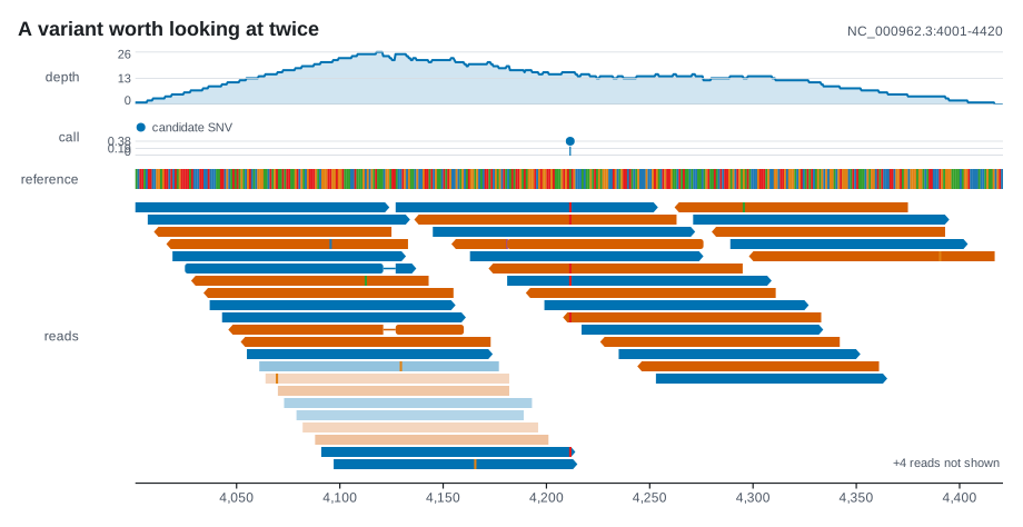
SAM

Aligned reads as text. A BAM is read as it is and a CRAM is piped from samtools view, as compressed and binary files shows; both arrive as these records.

@HD    VN:1.6  SO:coordinate
@SQ    SN:NC_002516.2  LN:6264404
read1  0  NC_002516.2  4001  60  3S5M2I4M1D6M  *  0  0  AAAGGGGGTTCCCCTTTTTT  *

Read by	--pileup; read::align::sam
Columns	2 FLAG (bit 4 unmapped, bit 16 reverse strand), 3 RNAME, 4 POS, 5 MAPQ (255 means none given), 6 CIGAR, 10 SEQ unless it is *
Ignored	1 QNAME, 7 RNEXT, 8 PNEXT, 9 TLEN, 11 QUAL, and the optional tags
Coordinates	1-based: POS 4001 starts the read at 0-based 4000
Skipped	unmapped records; records with * for a CIGAR
Refused	fewer than 11 columns; a POS of 0; a MAPQ above 255; a CIGAR that will not parse

M, = and X all arrive as matches: the track finds mismatches itself, by comparing SEQ with the reference --with-sequence gives it, or the figure's --sequence when there is no --with-sequence. I, D, N, S and H are read as themselves, and P, padding that moves along neither sequence, is dropped. Secondary and supplementary records are drawn like any other mapped record.

SAM with SA tags

Reads that aligned in pieces: a primary alignment, and an SA tag listing the others.

r1  0     chr1  1001  60  50M50S  *  0  0  *  *  SA:Z:chr1,3001,-,50M50S,60,0;
r1  2064  chr1  3001  60  50M50S  *  0  0  *  *  SA:Z:chr1,1001,+,50M50S,60,0;

Read by	--split-reads; read::split::reads
Columns	1 QNAME (the row's name), 2 FLAG, 3 RNAME, 4 POS, 5 MAPQ, 6 CIGAR, and the SA:Z: tag: rname,pos,strand,CIGAR,mapQ,NM for each other piece
Coordinates	1-based, both in column 4 and inside the tag
Skipped	secondary and supplementary records, whose pieces are already in the primary's tag; records with * for RNAME; reads in one piece; reads with a piece on another sequence; reads whose pieces disagree about the molecule's length
Refused	fewer than 11 columns; a POS of 0; a MAPQ above 255; an SA entry of fewer than five fields, or with a strand other than + or -; a CIGAR that will not parse or covers no reference bases

Each molecule's pieces come from its primary line and that line's tag, so a region-restricted samtools view still recovers the pieces outside the region, and a read whose primary alignment is missing is not read at all. The pieces are put in the order the molecule visited them, worked out from the clips and the strand rather than from reference position, which is what tells a read across an inversion from a read across a deletion.

SJ.out.tab

Splice junctions, as STAR counts them.

chr1  14830  14969  2  2  1  14  3  40

Read by	--junctions; read::junction::junctions
Columns	1 sequence, 2 first base of the intron, 3 last base of the intron, 4 strand (0 unknown, 1 forward, 2 reverse), 5 motif, 6 annotated (0 or 1), 7 uniquely mapping reads, 8 multi-mapping reads, 9 longest overhang
Coordinates	1-based and inclusive on the intron: the start moves back one and the end stays
With an index	read a window at a time, through the .tbi that tabix -s1 -b2 -e3 SJ.out.tab.gz writes
Refused	fewer than 9 columns; an intron start of 0; an intron that ends before it starts

The six motif codes fold to four (GT/AG, GC/AG, AT/AC and non-canonical), since each pair differs only in the strand, which has its own column. Multi-mapping reads are kept apart and never added to the unique reads the arc's thickness comes from. A run aligned without an annotation writes 0 in column 6 everywhere, which reads as every junction being new. A junction no uniquely mapping read crossed is kept, and the track holds it back and says how many it held back.

bedMethyl

Modified bases, one row per position per strand per modification, as modkit pileup writes them.

NC_000913.3  1000  1001  m  30  +  1000  1001  255,0,0  30  86.67  26  4  0  0  0  0  0

Read by	--methylation; read::methyl::sites
Columns	1 sequence, 2 start, 4 modification code, 6 strand, 10 valid coverage, 12 reads modified; the fraction is column 12 over column 10
Ignored	3 end, 5 score, 7 to 9, 11 percent modified (the same fraction, rounded), and 13 to 18
Coordinates	0-based, passed through: 1000 is the base 1,001 counted from 1
With an index	read a window at a time with --modification, through the .tbi that tabix -p bed calls.bed.gz writes; without it the file is read whole, since the codes offered are every code it holds
Skipped	rows counting another modification; rows with no valid coverage, which are positions nobody measured rather than 0% modified, and whose number --methylation prints on the band
Refused	fewer than 18 columns; a strand other than + or -, since a strand-combined pileup has no strand to draw; more reads modified than valid coverage

A file holding more than one modification code, such as m and h from a dual-mode run, needs --modification. The code is compared on its first field, so a motif run's m,CG,0 is m. Some tools write tabs up to column 10 and spaces after it, and that reads too.

The Bismark extractor file

Methylation calls one read at a time, as bismark_methylation_extractor writes them.

Bismark methylation extractor version v0.24.2
read_0001  +  chr7  57383000  Z
read_0001  -  chr7  57383012  z

Read by	--bisulfite; read::bisulfite::molecules
Columns	1 read name, 2 + or -, 3 sequence, 4 position, 5 call letter; the eight-column rows of Bismark's yacht output read too
Coordinates	1-based: the position moves back one
Skipped	the version line; calls in another context
Refused	a row that is not 5 or 8 columns; a column 2 other than + or -, or at odds with the case of the call; a call letter other than Z z X x H h U u; a position of 0

The call letter is both the context and the answer: Z and z are a CpG found methylated and unmethylated, X and x CHG, H and h CHH, U and u an unknown context. A file holding several contexts needs --context. Column 2 repeats the case of the letter; it is not the strand. Both mates of a pair carry one read name (a /1 or /2 ending is dropped) and are one row, one molecule, and where they disagree about a cytosine neither call is kept. A cytosine a molecule never covered is drawn as nothing, unlike one measured and found unmethylated.

SLOW5

The raw current of nanopore reads, as text. slow5tools view writes a BLOW5 file this way.

#slow5_version  0.2.0
#read_id    read_group  digitisation    offset  range   sampling_rate   len_raw_signal  raw_signal
read_1  0   8192    6   1467.61 4000    2400    432,434,436,450,433

Read by	--squiggle, or a .slow5 named on its own; read::series::squiggle
Columns	read_id and raw_signal, and digitisation, offset and range to put the signal in picoamperes, as (raw + offset) × range / digitisation
Coordinates	samples counted from 1
Skipped	every read but one: the one --read names, or the first
Refused	a read --read names that the file does not hold, with the reads it does

A file of plain numbers, one sample after another, is read too, as picoamperes already. POD5 and FAST5 are binary and are converted to SLOW5 first.

The bases the basecaller called come from its own record of the read, SAM or BAM as Dorado writes it with --emit-moves, named by --with-moves:

read_1  4  *  0  0  *  *  0  0  GGATCA  *  mv:B:c,5,1,0,0,0,0,1  ts:i:0

The move table, mv:B:c, is the stride and then a flag for each stride of samples, 1 where a new base begins, and ts:i is how many samples were trimmed from the start of the signal first. The record read is the one named as the signal's read, or one Dorado split out of it, which names it in pi:Z and says where it starts in sp:i; a record on the reverse strand is turned back into the order of the signal. Secondary and supplementary records are skipped, and a hard clipped record, a table that starts more or fewer bases than the read holds, or a record with no table are refused. A BAM is read from end to end, as a basecaller writes one neither sorted nor indexed.

Comparisons

PAF

Alignments between two sequences, as minimap2 writes them by default.

qry  4500  100  4400  +  ref  5000  200  4500  4100  4300  60

Read by	--synteny and --dotplot; read::align_pairs::blocks
Columns	1 query name, 3 query start, 4 query end, 5 strand, 6 target name, 7 target length, 8 target start, 9 target end, 10 residue matches, 11 alignment block length
Ignored	2 query length, 12 mapping quality, and the optional tag:type:value fields
Coordinates	0-based and half-open on both sequences, passed through: the one format here that needs no conversion
Skipped	rows about any other pair of sequences
Refused	fewer than 12 columns; a strand other than + or -; a target given two different lengths

The region names the query. Of the targets it aligns to, the one with the most rows is drawn (on a tie, the name first in alphabetical order), and the synteny track prints both names. A block's identity is column 10 over column 11, and a block length of 0 gives it none.

Gene neighbourhoods

The genes around one locus in several genomes: BED or GFF3 whose first column names the genome.

g1  100   900   dnaA  0  +
g1  1000  2100  dnaN  0  +
g2  150   950   A1    0  +
g2  1100  2200  N1    0  +

Read by	--loci, with --links; read::locus::loci
Columns	as BED or GFF3, told apart the same way, except that column 1 names the genome
Coordinates	as BED or GFF3
Skipped	column 1 names a genome and filters nothing; only the window filters
Refused	whatever BED or GFF3 refuses

Every genome in the file is a row, in the order first seen, so the file is what cat makes of one file per genome:

cat H37Rv.bed CDC1551.bed Erdman.bed > loci.bed

Every row is drawn against the one window as written, so give each genome's genes coordinates in a shared frame, such as positions within the neighbourhood; genes in whole-genome coordinates fall outside a small window. The gene names are what the homology table joins on, so each has to name one gene.

The homology table

Which gene matches which, between neighbouring genomes of a locus track.

dnaA  A1  98.5  800   12  0  1  800   1  800   0.0  1400
dnaN  N1  91.0  1100  99  0  1  1100  1  1100  0.0  1800

Read by	--links, after --loci; read::locus::links
Columns	1 query gene, 2 subject gene, 3 identity: BLAST tabular (-outfmt 6, or 7 with its comment lines) as DIAMOND and others write it, or just two or three columns
Ignored	columns 4 to 12 of BLAST tabular
Coordinates	none: a homology names two genes, and where they are is in the loci file
Skipped	rows naming a gene no locus has; two genes in one genome; genomes not next to each other in the stack; repeats of a pair already seen
Refused	a row that is not 2, 3, or 12 or more columns; an identity outside 0 to 100 (0 to 1 for a fraction); an identity column that could be either unit; a gene name that more than one gene answers to

An empty identity, ., NA, na, N/A and * mean none was reported. Left to itself, a file with any identity above 1 is read as percentages, and one whose every identity is at or below 1 is refused until --identity says percent or fraction. Names are matched exactly, and a file in which none match is refused by the command.

The InterProScan table

Protein domains, as InterProScan writes its tab-separated output.

P00533  md5  1210  Pfam  PF07714  Protein tyrosine kinase  712  979  1e-70  T  01-01-2026

Read by	--domains; read::domain::architectures
Columns	1 protein, 3 protein length, 4 analysis, 5 signature accession, 6 signature description, 7 start, 8 stop
Ignored	2 MD5, 9 score, 10 status, 11 date, and 12 to 15 (InterPro entry, GO terms, pathways)
Coordinates	1-based and inclusive, in residues: the start moves back one and the stop stays
Skipped	rows from another analysis; column 1 names a protein and filters nothing
Refused	a line with no tab; fewer than 11 columns; a length of 0; a protein given two different lengths; a start of 0; a stop before its start

The example is spaced out to be read; the file itself must be tab separated, because column 6 is a sentence and splitting it on spaces would shift every column after it. The region is a range of residues, such as P00533:1-1,210, and every protein in the file is a row on that shared axis. A row's backbone is drawn to the length in column 3, not to its last domain, and each domain is labelled with its description, or its accession where the description is empty, . or -. A file from several analyses, such as Pfam, PANTHER and Gene3D, needs --analysis.

Gubbins clade blocks

Stretches of a reference carried by a named set of taxa, as the GFF3 that Gubbins writes for recombination.

SEQUENCE  GUBBINS  CDS  1531  1670  0.000  .  0  node="N7";taxa="s1 s2 s3";

Read by	--clades, with --with-tree; read::clade::blocks
Columns	1 sequence, 4 start, 5 end, 9 attributes: taxa, which is required, and the block's name from node, Name or ID
Ignored	2 source, 3 type, 6 score, 7 strand, 8 phase
Coordinates	1-based and inclusive, as GFF3
Skipped	a taxon named twice in one block; rows on another sequence only when the file names more than one
Refused	fewer than 9 columns; a start of 0; an end before its start; a row with no taxa, or with an empty one

Gubbins writes SEQUENCE in column 1 whatever the reference was called, so a file naming one sequence is read whatever it calls it; a file naming several is a whole genome, and the region picks among them. taxa is split on spaces, tabs and commas, its quotes removed, and each name percent-decoded after the split, then joined to the tree's tips. The list holds spaces, so the file has to be tab separated, as Gubbins writes it.

Metadata

The sample sheet

What is known about named rows, drawn as strips beside a track's rows.

sample  lineage  host    depth  drug
S001    L4       human   72.5   true
S002    L2       bovine  61.0   false
S003    L4       NA      48.2   true
S004    L1       human   NA     false

Read by	--traits, after --matrix, --msa, --snps, --clades, --domains, --loci or --tree; read::sheet::sheet
Columns	a required header, whose first field names the name column and every other field an attribute; then one row per name
Coordinates	none: the strips sit beside the rows and do not move with the region
Refused	an empty file; a header of one column; an empty or repeated column name; a row whose field count differs from the header's; an empty or repeated name

A field is a number when it parses as one, true or false when it spells one, and text otherwise. A column whose every value is a number is drawn on a colour ramp; any other column gets a colour per level, and a shape as well once it has more than six levels, unless --colors gives its levels colours of your own (see Sample sheets beside the rows). An empty field (tab-separated files only), ., NA and NaN are missing and drawn as an empty outline, so a column whose levels really include NA, a continent code for instance, loses them to missing. The first line is always the header, and the join to the track's rows is by exact name.

Where next

• Command line

  Which flag takes which file, and the rest of the grammar.

• Coordinates

  Why the conversions above are the conversions they are.

• Recipes

  These readers at the end of real pipelines.