Phylogenetics
Read a tree with its metadata intact and draw it on branch length or calendar time, in rectangular, circular or unrooted coordinates, with support, selection, clades and sample traits on it. Every drawing choice leaves the tree itself as it was.
Command line or library
--tree reads Newick or NEXUS and reaches metadata strips (--traits),
branch colour (--color-by), --projection, --support-style,
--support-from, --no-scale-bar, --shape, folding (--max-rows),
--focus, --mutations and --highlight; every flag is in
Command line. Calendar time, rerooting, branch geometry, dN/dS,
node glyphs and the ancestral and selection layers are library only.
From your files to a figure
The eight steps most figures of a tree take, each a few lines. Every one starts
from a tree read with Tree::parse and a plot started with plot_tree(),
which names no place and draws no ruler, since a tree's x is a branch length
and not a position. Each goes in a main that returns
Result<(), Box<dyn std::error::Error>>, so ? works on every call, and each
goes on from the one before it: the tree the first reads and the sheet the
third reads are the ones the rest draw.
Read the tree
Tree::parse reads Newick, as IQ-TREE and RAxML write it, and NEXUS, as BEAST,
MrBayes and FigTree do, whichever the file is, and keeps the BEAST, NHX and
IQ-TREE annotations on it. A file of several trees gives its first, and
Tree::parse_all gives every one. A tree that does not parse says at which
character it broke.
Draw it, with its support
use karyon::{plot_tree, SupportStyle};

plot_tree()
    .add_tree(tree)
    .adjust(|track| {
        track
            .support_style(SupportStyle::Labels)
            .support_threshold(70.0)
    })
    .save("tree.svg")?;
A phylogram with branch lengths draws its scale bar by itself. Support is read
once for the whole tree, so 70.0 and 0.7 are the same threshold, and a
threshold hides only what a support style would have drawn. A tree out of BEAST
or MrBayes keeps its support in an annotation, which .support_from("posterior")
or .support_from("prob") reads; IQ-TREE's 95.3/88 is read as two values,
the last drawn.
Put what you know about the samples beside the tips
use karyon::{plot_tree, Sheet, Traits};

let sheet = Sheet::parse(&std::fs::read_to_string("samples.tsv")?)?;

plot_tree()
    .add_tree(tree)
    .adjust(|track| track.traits(Traits::from_sheet(&sheet).strips(["lineage", "country"])))
    .add_key()
    .save("strips.svg")?;
A sheet is a tab-separated table with a header, the names in its first column
and one column per thing known about them. traits joins it to the tips by
name, draws each column named in strips as a strip, and says under the tree
which tips it has no row for; .join() on the track gives what matched and
what was left out on both sides. Each column starts on a stretch of the palette
of its own, in the order of the sheet, so a value added to one column later
does not repaint another, and a value is one colour in every figure drawn from
the sheet. add_key() keys every strip at the foot of the figure, in the
colours it drew.
The palette has six colours. A column with more values than that is drawn as shapes, each value a colour and a shape of its own, and the figure says so under the tree; so does one whose values run into the colours of the strip beside it. To keep it a strip, give its values colours of your own, as a field that knows its lineages by colour already would:
let traits = Traits::from_sheet(&sheet)
    .strips(["lineage", "country"])
    .colors("country", [
        ("China", "#1b9e77"), ("India", "#d95f02"), ("Kenya", "#7570b3"),
        ("Peru", "#e7298a"), ("Portugal", "#66a61e"), ("Spain", "#e6ab02"),
        ("Vietnam", "#666666"),
    ]);
or draw the figure in a theme with more colours, with plot_tree().theme(theme)
and a longer theme.palette: which values are shapes is decided in the theme
the figure is drawn in. colors may come before strips as well as after, and
reaches the branches of a tree coloured by the column with no strip of it
beside them. From the command line the same colours are a figure option:
karyon tree.nwk --traits samples.tsv --columns lineage,country \
  --colors 'country=China:#1b9e77,India:#d95f02,Kenya:#7570b3,Peru:#e7298a' \
  --colors 'country=Portugal:#66a61e,Spain:#e6ab02,Vietnam:#666666'
Colour the branches and fold a clade
use karyon::{plot_tree, NodeRef, Traits};

plot_tree()
    .add_tree(tree)
    .adjust(|track| {
        track
            .traits(Traits::from_sheet(&sheet))
            .color_by("lineage")
            .collapse(NodeRef::holding("lineage", "L4"))
    })
    .add_key()
    .save("folded.svg")?;
A sheet joined with no strips draws no strip, and still gives each tip its
values, which is all color_by and the fold need; name lineage in strips
too for a strip beside the branches. color_by colours each branch by a column
of the sheet or an annotation of the file, and a clade whose tips agree takes
their colour too; a column of the sheet colours the branches as its strip
does, drawn or not, so L1 is one colour in every figure of a set. A clade is
named as you would name it: NodeRef::holding("lineage", "L4") is the smallest
clade holding every L4 tip, NodeRef::mrca(["S01", "S07"]) the smallest
holding two tips, and a name or an index works as it is. A clade that holds
tips it was not named for is folded all the same, and the tips are said under
the tree. A folded clade is a wedge in the colour of its branches, named by
the value it was folded by, as L4 (16 tips), by a name of its own where it
has one, and otherwise by its first tip and how many more it holds, as
S26 +15 more; its tooltip gives its first and last tips.
Draw it as a circle
plot_tree()
    .add_tree(tree)
    .adjust(|track| {
        track
            .traits(Traits::from_sheet(&sheet).strips(["lineage"]))
            .circular()
    })
    .add_key()
    .save("circle.svg")?;
The strips become rings around the tips, keyed the same way. One ring is named by the key; two or more are named across the top as well, inside out. Change the projection, not the tree has the fans, the inward trees and the unrooted drawing.
Put an alignment in the order of the tree
use karyon::{plot_alignment, read, MsaSequence};

let rows: Vec<MsaSequence> = read::seq::alignment(&std::fs::read_to_string("aln.fasta")?)?
    .into_iter()
    .map(|(name, bases)| MsaSequence::new(name, bases))
    .collect();

plot_alignment(rows)
    .adjust(|track| track.tree(tree))
    .add_key()
    .save("alignment.svg")?;
An alignment is placed by its columns, so plot_alignment plots over them, as
many as its longest row has, with a ruler that counts them. tree sorts
the rows by descent and draws the tree beside them, cut to the rows there are;
a tip with no row is counted under the tree, and a row the tree does not name
stays at the bottom. Only the bases that differ from the consensus are
painted, which is what makes forty rows of a long alignment readable, and
add_key() says which colour is which base; .display(MsaDisplay::Bases)
paints every base. Forty rows are drawn at most, and .max_rows(None) draws
them all.
Put two trees face to face
use karyon::plot_tree;

let right = Tree::parse(&std::fs::read_to_string("tree2.nwk")?)?;

plot_tree()
    .add_tanglegram(tree, right)
    .adjust(|track| track.names("tree", "tree2").untangle())
    .save("tanglegram.svg")?;
Each tip is joined to its twin, so a disagreement is a crossing, and untangle
turns clades to lower the count without changing either tree.
Draw it against the years
plot_tree()
    .add_tree(tree)
    .adjust(|track| track.time("date").time_unit("year"))
    .save("dated.svg")?;
time places every node on a date each tip carries, a decimal year or a date
written as 2020-03-15, with the years along an axis and year as its title.
A tree dated in BEAST heights, each node's age back from the most recent tip,
is turned into dates first, given that tip's date:
let mut tree = Tree::parse(&std::fs::read_to_string("mcc.tree")?)?;
tree.date_from_height("height", 2021.5, "date");
A tip with no date draws the tree by branch length and says why under it, as every request a tree cannot carry out does.
Read annotations instead of flattening them
use karyon::{AnnotationValue, Tree};

let tree = Tree::parse(
    "[&R] (sample_A[&date=2024.25,country=Peru,selected=true]:0.2,\
            sample_B[&date=2024.50,country=Spain]:0.3);",
)?;
let sample = tree.node_named("sample_A").unwrap();

assert_eq!(
    tree.annotation(sample, "date").and_then(AnnotationValue::as_number),
    Some(2024.25),
);
assert_eq!(tree.rooted(), Some(true));
Values keep their type: numbers, text, booleans and brace-delimited lists
become AnnotationValue::Number, Text, Boolean and List, read back with
as_number, as_text and as_bool.
| Reader | Reads | Annotations |
|---|---|---|
Tree::parse |
Newick or NEXUS, whichever the text is; the first tree of several | kept |
Tree::parse_all |
every tree of a Newick or NEXUS text | kept |
Tree::parse_annotated_newick |
Newick with BEAST [&key=value] or NHX [&&NHX:key=value] comments |
kept and typed, on the node written before them; [&R] and [&U] set rooted() |
Tree::parse_nexus |
the first tree of a Nexus trees block |
kept; the translate table renames the tips |
Tree::parse_newick |
Newick | discarded |
An internal label that reads as a number is taken as support, anything else as
a name, and so is a label in quotes, as '100'. Several numbers parted by /,
as IQ-TREE writes 95.3/88, are support: the last is drawn and each is kept as
support_1, support_2, which support_from can draw instead. annotations_mut adds metadata from Rust. Node indices survive
rotating, ladderising and rerooting; subtree and Tree::collapse renumber
them, since each leaves a compact tree.
Changes on branches
use karyon::{Mutations, Tree};

let tree = Tree::parse(
    r#"((a[&muts="A123T,S:D614G"]:0.1,b:0.2)[&muts="C241T"]:0.3,c:0.4);"#,
)?;
let changes = Mutations::read(&tree, "muts");

assert_eq!(changes.distinct(), 3);
// C241T happened once, above a and b: the clade and both tips carry it.
assert_eq!(changes.carriers(&tree, "C241T").len(), 3);
A change belongs to the branch above the node that carries it, so carriers
answers with the whole subtree below, and a change that happened twice answers
with both. Changes are read from a quoted list or one in braces, spelled
A123T, S:D614G or either with an nt: or aa: prefix; anything else is
skipped, not guessed, and unread counts it. --carrying marks and colours
the carriers, and refuses a change the tree does not carry.
Draw time, branches and sample traits together
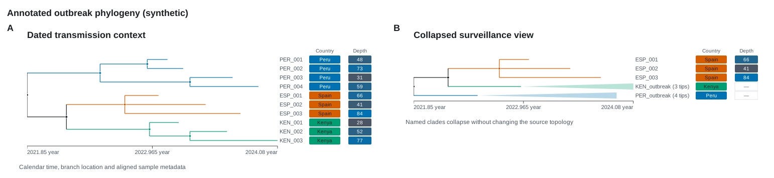
use karyon::{plot_tree, TraitColumn, TreeTrack};

let track = TreeTrack::new(tree)
    .time("date")
    .time_unit("year")
    .color_by("country")
    .show_nodes(true)
    .trait_column(TraitColumn::categorical("country").label("Country"))
    .trait_column(TraitColumn::continuous("depth").label("Depth"));

plot_tree().add_track(track).save("outbreak.svg")?;
time(key) places every node on an annotation, here a decimal year, or a date
written as 2020-03-15, with a calendar axis underneath and time_unit as its
title. The command line has no time axis and draws branch length instead.
color_by(key) uses a ramp when every value in the tree is a number and the
categorical palette otherwise. A branch with no value takes its nearest
annotated ancestor's, or failing that the value all its descendants share, so
a clade of one lineage is coloured whole and not only at its tips.
Each TraitColumn is one strip beside the tips. Levels are coloured in the
order the tree meets them, counted over the whole tree, so folding a clade does
not repaint the rest. A column that came from a sample sheet carries the
sheet's order instead (TraitColumn::levels), so a lineage is the colour here
that it is beside every other track the sheet is drawn with. legend(&theme)
hands back a key read off the same count as the branches and the strips, and
Figure::key() gathers it in the figure's own theme, so a dark figure is keyed
in the colours it drew. Each entry copies its mark: a symbol column is keyed
with its shapes and a binary one with the two dots it draws. A
missing value is an empty outline whose tooltip says missing, never a zero, and
show_values(false) drops the text inside the cells.
What a time tree needs
Every tip needs a finite number under the time key. Internal nodes without
one are inferred from their children and branch lengths, subtracting lengths
for dates and adding them for heights before present:
use karyon::{TimeDirection, TreeTrack};

let track = TreeTrack::new(tree)
    .time("height")
    .time_direction(TimeDirection::Decreasing)
    .time_unit("years BP");
time_direction, time_unit and show_time_axis do nothing without
time, and count the same written before it or after it. If a tip has no
value the track falls back to its ordinary layout, without a time axis, and
says why under the tree. Where a missing date must be an error instead,
check Tree::time_layout first: it returns None. Heights can be turned
into calendar dates instead, given the most recent tip's date, with
Tree::date_from_height("height", 2021.5, "date").
Change the projection, not the tree
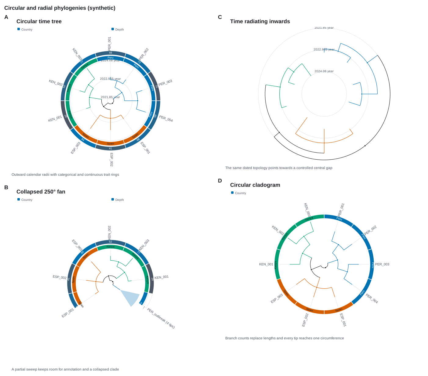
use karyon::{RadialDirection, TraitColumn, TreeTrack};

let outward = TreeTrack::new(tree.clone())
    .time("date")
    .color_by("country")
    .trait_column(TraitColumn::categorical("country").ring_width(12.0))
    .circular()
    .radial_start(-90.0)
    .radial_size(520.0);

let inward_fan = TreeTrack::new(tree)
    .time("date")
    .fan(250.0)
    .radial_start(-215.0)
    .radial_direction(RadialDirection::Inward)
    .inner_radius(0.32);
A projection changes coordinates and nothing else: lengths, dates, annotations and tip order are not recomputed. In a circle, time ticks become concentric guides, trait columns become rings and a collapsed clade becomes a wedge.
| Builder | Effect | Default |
|---|---|---|
circular() |
a full circle | |
fan(degrees) |
a partial clockwise sweep, 10 to 359 degrees | |
radial_start(degrees) |
where the first tip sits, clockwise from three o'clock | -90, twelve o'clock |
radial_sweep(degrees) |
the sweep, 10 to 360 degrees | 360 |
radial_direction(RadialDirection::Inward) |
tips towards the centre, root at the rim | Outward |
inner_radius(fraction) |
a central gap, 0 to 0.85 of the radius | 0.08 |
radial_size(pixels) |
fixes the diameter | sized to the tip names |
projection(TreeProjection::Circular) |
circular coordinates, other settings kept | Rectangular |
fan, radial_start, radial_sweep, radial_direction and inner_radius
also switch the track to circular coordinates. Left alone, a circle grows until
neighbouring tip names clear each other, from 440 pixels up to the width of the
figure; past that, use a wider figure, fewer rows or
show_tips(false).
A full circle suits a figure about topology and metadata, a fan leaves a quiet sector for a key, and an inward tree puts the early branches on the rim. None of them has rows, so keep the rectangular projection when each tip is read against the row beside it.
Without a root
unrooted() centres the tree on the node that splits its tips most evenly,
gives every tip an equal share of the angle, and leaves the file's root where
it is in the data. A phylogram keeps branch lengths and a cladogram gives each
edge one unit; unrooted_start rotates the drawing and unrooted_size fixes
its height. Names sit at their branch ends until they would touch, then gather
onto a ring with a leader each, as they always do when trait rings are drawn.
There is no time axis or root diamond, because both need a root.
Layer metadata around the tree
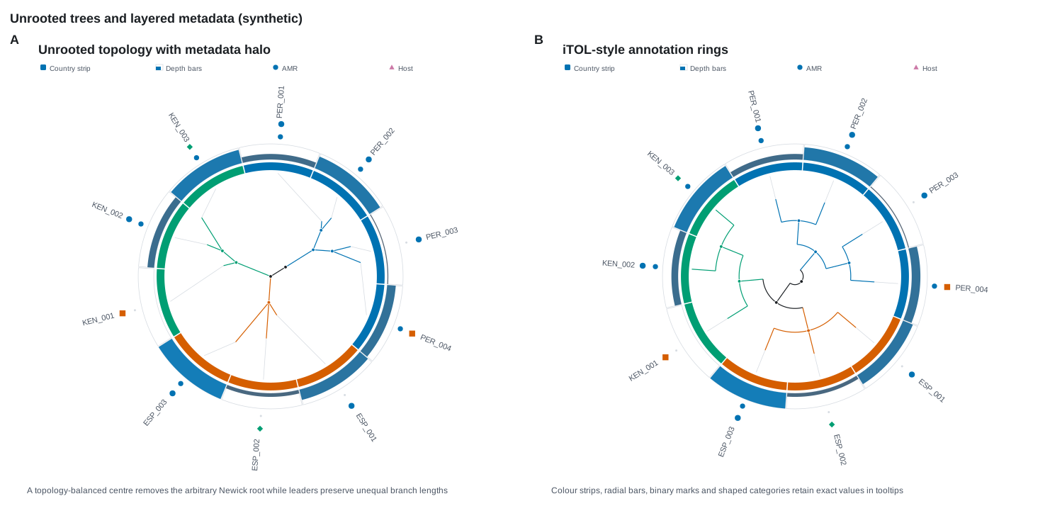
use karyon::{TraitColumn, TreeTrack};

let view = TreeTrack::new(tree)
    .unrooted()
    .color_by("country")
    .trait_column(TraitColumn::categorical("country").label("Country"))
    .trait_column(TraitColumn::bar("depth").label("Depth"))
    .trait_column(TraitColumn::binary("resistant").label("AMR"))
    .trait_column(TraitColumn::symbol("host").label("Host"));
A TraitColumn is one dataset: a column beside a rectangular tree, a ring
around a circular or unrooted one, with the same key and tooltip either way.
| Constructor | Beside a rectangular tree | Around a circular or unrooted tree | Takes |
|---|---|---|---|
TraitColumn::categorical(key) |
colour strip | ring of colour | any value |
TraitColumn::continuous(key) |
heatmap cell | ring of heatmap sectors | a finite number |
TraitColumn::bar(key) |
horizontal bar | radial bar | a finite number |
TraitColumn::binary(key) |
presence mark | ring of marks | a boolean, or a number where zero is absent |
TraitColumn::symbol(key) |
coloured shape | ring of shapes | any value |
A binary column never guesses text into true or false, and a missing value
stays an outline in every mark. width sizes a column and ring_width a ring,
2 to 24 pixels; trait_categorical, trait_bar and their siblings on
TreeTrack add columns with their defaults. --traits picks the mark from the
values: numbers get a ramp, more than six levels get symbols, anything else a
colour strip. A strip whose levels outnumber the palette's colours is drawn as
symbols however it was built, and each column of words on a tree takes its own
stretch of the palette, as a sheet's columns do, so a lineage and a country are
never one colour while each fits its stretch.
Choose a tree geometry
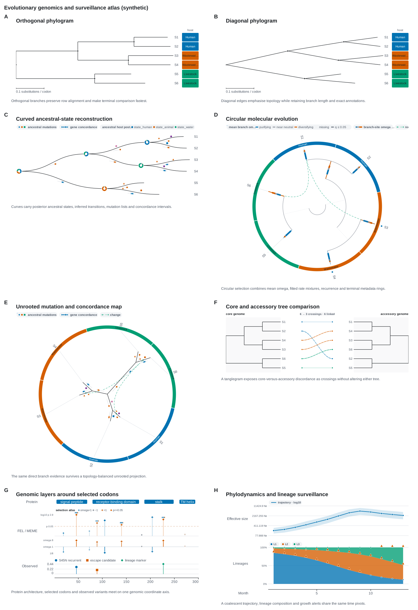
use karyon::{BranchGeometry, TreeTrack};

let aligned = TreeTrack::new(tree.clone()).branch_geometry(BranchGeometry::Orthogonal);
let topology = TreeTrack::new(tree.clone()).branch_geometry(BranchGeometry::Diagonal);
let presentation = TreeTrack::new(tree).branch_geometry(BranchGeometry::Curved);
| Geometry | Best for | Watch for |
|---|---|---|
Orthogonal, the default |
aligned tip rows, events and dense metadata columns | parent risers can dominate a very unbalanced tree |
Diagonal |
topology and the direction of change | weaker alignment between a node and its descendants |
Curved |
annotated internal nodes and presentation figures | keep node glyphs small so curves do not cross them |
| circular | many tips with metadata rings | root and tip order still carry meaning |
| fan | radial context with a quiet sector | a partial sweep gives tips unequal directions, not unequal weight |
| unrooted | split structure without the file's root | cannot show the direction of time |
branch_geometry affects the rectangular projection only, and never reroots,
ladderises or rotates. The rest of the sheet is a tanglegram (F), a selection
scan (G), and the evolution and surveillance tracks
(H).
Show support, events and distance
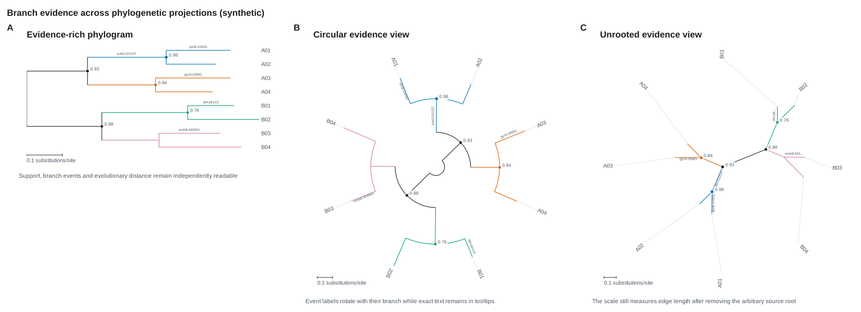
Support, events and branch length answer different questions, so each has a channel of its own.
SupportStyle::None, the default, keeps support in the tooltips; Symbols
scales a marker by it, Labels prints it and SymbolsAndLabels does both.
support_threshold hides weaker values in either convention, 0.70 or 70,
and a label keeps the value as the file wrote it. The convention is read once
for the whole tree: one value above one puts every value out of a hundred, so a
clade at 1 on a bootstrap tree is one per cent and not full support.
branch_labels(key) writes a node's own annotation along its incoming branch
and never inherits, so a mutation is not repeated on every descendant. Labels
turn with their branch, and one that does not fit is shortened and kept whole
in its tooltip.
scale_bar() picks the largest 1, 2 or 5 step within a fifth of the tree's
span; scale_bar_length sets the length and scale_bar_unit names the unit.
Cladograms and time trees get no bar, since their axis is not branch length.
Ancestral states, events and intervals
use karyon::{AncestralStateLayer, BranchEventLayer, BranchIntervalLayer, TreeTrack};

let reconstruction = TreeTrack::new(tree)
    .ancestral_states(
        AncestralStateLayer::new(["state_human", "state_animal", "state_water"])
            .label("ancestral host posterior")
            .confidence(0.72),
    )
    .branch_event_layer(BranchEventLayer::new("mutations").maximum_events(6))
    .branch_interval(
        BranchIntervalLayer::new("gcf", "gcf_low", "gcf_high")
            .label("gene concordance")
            .range(0.0, 1.0)
            .threshold(0.70),
    );
A reconstruction yields three different things, and folding them into one branch colour would lose both ownership and uncertainty. Each layer keeps one apart, in every projection, and none inherits values (panel C of the geometry sheet):
AncestralStateLayer: the state probabilities as a donut on each internal node, and a mark where the most probable state changes, only when both ends reachconfidence, 0.70 by default.BranchEventLayer: one mark per event on its own branch; a brace-delimited list is several, up tomaximum_events, 8 by default.BranchIntervalLayer: an estimate and its bounds on a small axis, 0 to 1 unlessrangesays otherwise; a reversed interval is dropped, not repaired.
Choose the root
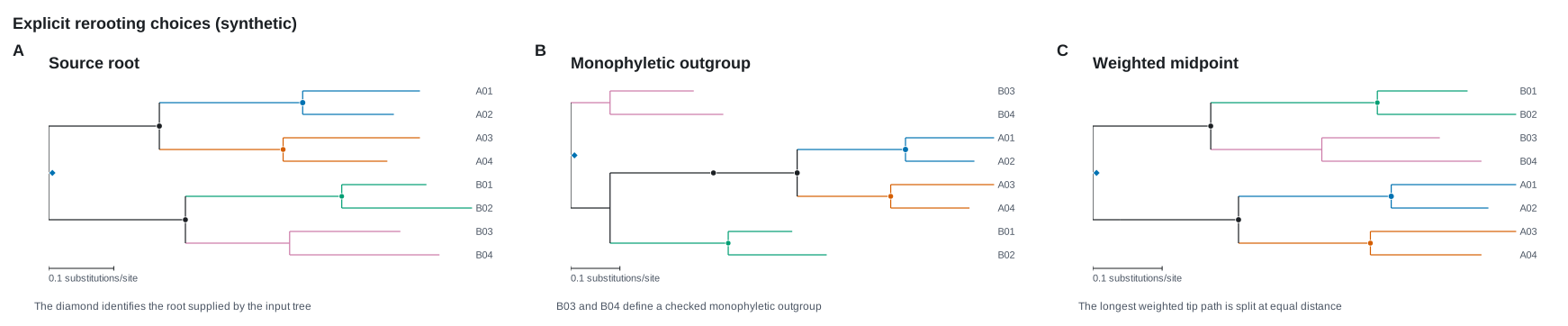
use karyon::TreeTrack;

let by_clade = TreeTrack::new(tree.clone()).reroot_named("lineage_4");
let by_outgroup = TreeTrack::new(tree.clone()).reroot_outgroup(["B03", "B04"]);
let by_midpoint = TreeTrack::new(tree).reroot_midpoint();
Rerooting keeps every tip-to-tip distance and keeps support on its split; a root inside a branch adds one node. A diamond marks the new root in rectangular and circular coordinates.
| Builder | Accepts | Roots at |
|---|---|---|
reroot(node) |
an internal node: its index, its name, or a NodeRef picking it by its tips or a value |
that node |
reroot_named(name) |
an internal node's exact name | that node |
reroot_outgroup(names) |
existing, distinct tip names forming exactly one clade | halfway along the branch above that clade |
reroot_midpoint() |
a tree whose every branch has a finite, non-negative length | halfway along the longest tip-to-tip path |
show_root(false) |
hides the diamond, keeps the root |
A request the tree cannot meet leaves the builder's tree unchanged, and the
band says so in a line under the tree: not rerooted: no tip is named B3. The
same goes for a fold or a highlight that names a node the tree does not have,
a key no node carries, a time axis some tip has no date for and a support
threshold with no support style, and TreeTrack::warnings() hands the same
lines to a caller that would rather stop; the command line prints them. A fold
or a highlight asked for before a reroot follows its clade through it, by its
tips, and one the new root splits is said rather than drawn. Where a failed
reroot must be an error, call the operation on the Tree and check its
result:
use karyon::TreeTrack;

let b03 = tree.node_named("B03").unwrap();
let b04 = tree.node_named("B04").unwrap();
let root = tree.reroot_outgroup(&[b03, b04]).ok_or("the outgroup is not one clade")?;
let track = TreeTrack::new(tree).show_root(true);
Show dN/dS around the neutral point
use karyon::TreeTrack;

let view = TreeTrack::new(tree)
    .dnds("omega")
    .dnds_label("Branch dN/dS (ω)")
    .dnds_neutral_band(0.9, 1.1)
    .dnds_saturation(4.0)
    .dnds_significance("q", 0.05)
    .branch_labels("amino_acid_change");
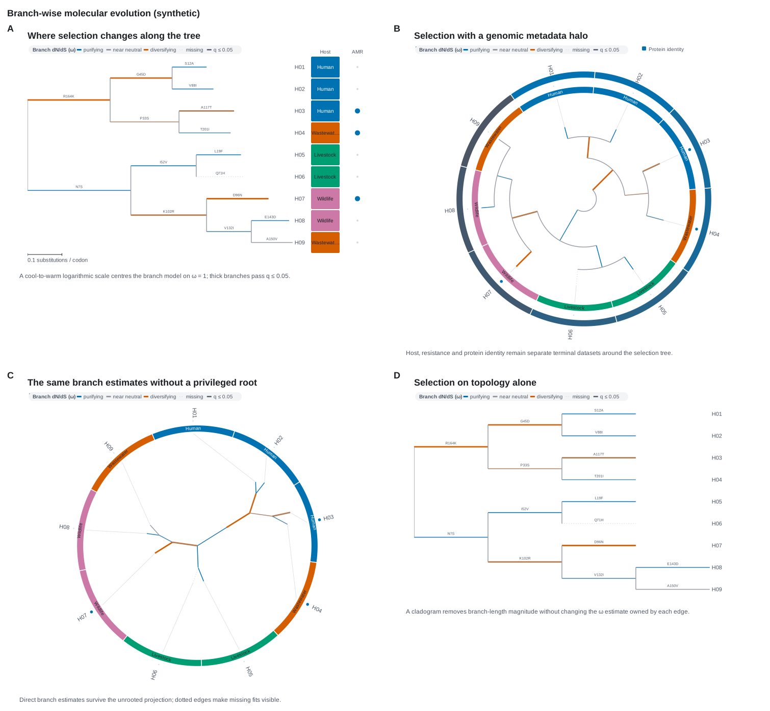
dnds(key) colours each branch by its own ω on a diverging scale fixed at
ω = 1, whatever range was observed, and never inherits it. Cool is below the
neutral band, 0.95 to 1.05 by default, grey inside and warm above. Strength
follows abs(log2(ω)) and saturates symmetrically: with
dnds_saturation(4.0), ω ≤ 0.25 and ω ≥ 4 are the strongest. Zero is the
strongest purifying value; a negative, non-finite or missing estimate is a
dotted branch, not a zero.
dnds_significance(key, maximum) thickens a branch whose own test value is at
most maximum, so width carries the evidence and colour the effect size.
dnds and color_by both colour the branches, so where both are set the dN/dS
colouring is drawn, whichever was written first, and the band says the other
was not. The other dnds_ settings do nothing without dnds and count the
same written before it or after it. The
estimates come from upstream: karyon computes no dN, dS,
tests or corrections, and calls ω above the neutral band diversifying, not
proof of positive selection.
Keep rate classes and site evidence apart
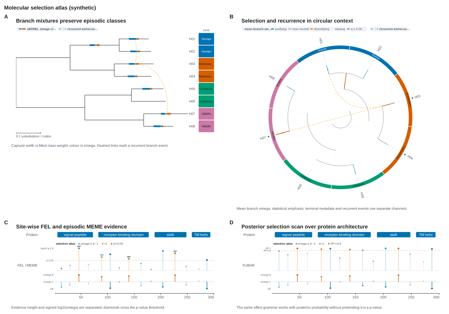
A branch-site model fits several ω classes to one branch, and a single mean would hide them.
use karyon::{BranchRateMixture, HomoplasyLayer, TreeTrack};

let rates = BranchRateMixture::new(
    ["omega_1", "omega_2", "omega_3"],
    ["weight_1", "weight_2", "weight_3"],
)
.label("aBSREL ω classes")
.neutral_band(0.9, 1.1)
.saturation(6.0);

let view = TreeTrack::new(tree)
    .branch_rate_mixture(rates)
    .homoplasy_layer(HomoplasyLayer::new("amino_acid_change").label("recurrent amino-acid change"));
BranchRateMixture pairs rate keys with weight keys in order and draws a
capsule on each branch: segment length is the class weight, segment colour the
class ω on the dnds scale. The tooltip keeps the weights as given, and a
class with an invalid rate or weight is left out.
HomoplasyLayer joins the branches that carry the same annotation with dashed
curves, once it is on minimum_occurrences branches (2 by default), and draws
at most maximum_connections curves (96), so a common event cannot turn a
dense tree into a web. A brace-delimited list is read one event at a time, as
BranchEventLayer reads it, so a branch carrying {S45N,E88K} is joined to
every branch carrying either. It calls them recurrent events: whether they are
convergence or reversal is for the analysis to settle.
Site models belong on the coordinate axis:
SelectionTrack draws each codon's
evidence above its signed log2(ω), so a well supported purifying site never
looks like a positive-selection hit.
Collapse, highlight and annotate clades
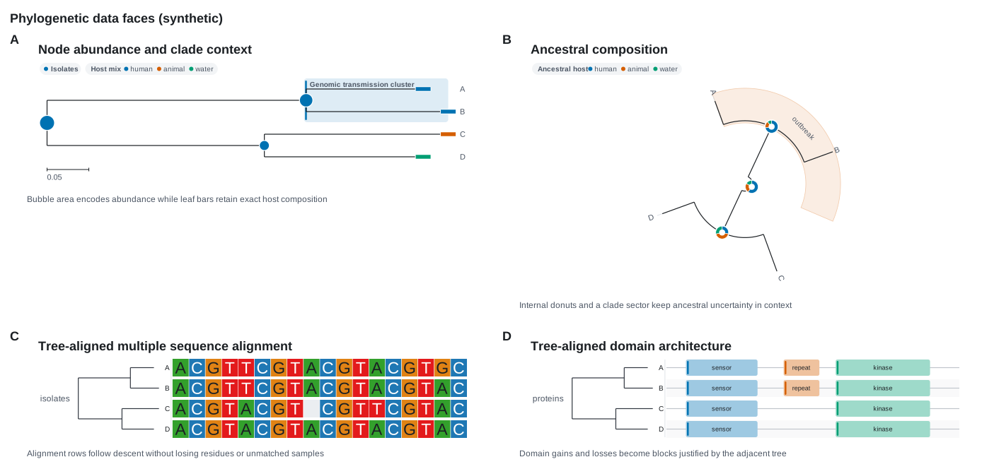
use karyon::{CladeHighlight, NodeGlyph, NodeGlyphTarget, TreeTrack};

let track = TreeTrack::new(tree)
    .node_glyph(
        NodeGlyph::bubble("isolates")
            .label("Isolate count")
            .target(NodeGlyphTarget::Internal),
    )
    .node_glyph(
        NodeGlyph::donut(["human", "animal", "environment"])
            .label("Host probability")
            .target(NodeGlyphTarget::Internal),
    )
    .clade_highlight(
        CladeHighlight::new("outbreak")
            .label("Transmission cluster")
            .opacity(0.12),
    );
CladeHighlight shades a clade in any projection and gives its tip count in
the tooltip. It takes the clade as collapse does, by index, by name, or as a
NodeRef picking it by its tips or a value; --highlight does it by name. NodeGlyph
draws numeric node annotations as small plots:
| Constructor | Needs | Draws |
|---|---|---|
NodeGlyph::bubble(key) |
one finite, non-negative number | a circle whose area follows it |
NodeGlyph::pie(keys) |
one such number per key | filled sectors |
NodeGlyph::donut(keys) |
one such number per key | annular sectors |
NodeGlyph::stacked_bar(keys) |
one such number per key | a compact horizontal bar |
A composition is normalised to fill its glyph, and the tooltip keeps every
value as given. NodeGlyphTarget::Internal or Leaves keeps a dataset where it
means something, and a node missing a key gets no glyph rather than a zero.
Collapse a clade
use karyon::{NodeRef, TreeTrack};

let by_name = TreeTrack::new(tree.clone()).collapse("PER_outbreak");
let by_tips = TreeTrack::new(tree.clone()).collapse(NodeRef::mrca(["PER_001", "PER_004"]));
let by_value = TreeTrack::new(tree).collapse(NodeRef::holding("country", "Peru"));

assert!(by_value.warnings().is_empty());
TreeTrack::collapse folds a clade into a triangle and leaves the tree
untouched; Tree::collapse removes the descendants from the data. The clade is
named as a reader names one: by its name, as the smallest clade holding some
tips, as ggtree's MRCA does, or as the clade of every tip carrying a value. A
clade found that way that also holds tips it was not named for is folded all
the same, and the tips are said under the tree. A folded
row shows a metadata value only when every tip inside agrees on it: tips that
differ, or one tip with nothing recorded, leave the cell empty.
Operation on Tree |
Effect |
|---|---|
ancestors, descendants, clade_size, leaves, leaf_names |
query the rooted topology |
mrca(&nodes) |
the most recent common ancestor of a non-empty set |
rotate(node) |
reverse one split without changing its clades |
ladderize(largest_first) |
order every split by tip count, ties kept in file order |
reroot, reroot_outgroup, reroot_midpoint |
reorient, as above |
subtree(node) |
copy one clade into a tree of its own |
collapse(node) |
replace a clade's descendants with one tip |
All of them walk the tree without recursion, so a deep tree cannot overflow the stack. For stretches of sequence carried by whole clades, see CladeTrack.
Sort rows by descent
use karyon::{DomainArchitecture, DomainFeature, DomainTrack, MsaTrack};

let alignment = MsaTrack::new(sequences).tree(tree.clone()).tree_width(110.0);

let architectures = vec![
    DomainArchitecture::new("sample_A", 300)
        .feature(DomainFeature::new(20, 110).label("sensor"))
        .feature(DomainFeature::new(170, 260).label("kinase")),
];
let domains = DomainTrack::new(architectures).tree(tree).tree_width(110.0);
MsaTrack, DomainTrack, SnpTrack, MatrixTrack and GenotypeTrack take a tree, draw it beside their rows and sort the rows to match, so a clade's shared changes form one block (panels C and D above). Rows match tips by exact name, and a row the tree does not name stays at the bottom rather than disappearing.
Compare two trees
use karyon::{TangleLabels, TangleTieStyle, TanglegramTrack};

let comparison = TanglegramTrack::new(core, accessory)
    .names("core genome", "accessory genome")
    .labels(TangleLabels::Both)
    .tie_style(TangleTieStyle::Curved)
    .color_by("ward")
    .untangle();

assert!(comparison.crossings() <= comparison.initial_crossings());
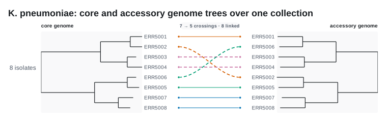
Each tip is joined to its twin in the other tree, so a disagreement is a
crossing. untangle rotates free clades on both sides and keeps only rotations
that strictly lower the count. It changes no clade or length and is
deterministic, but it is a local search, not a guaranteed minimum. The summary
gives the crossings before and after, the linked tips and the unmatched ones.
Crossing ties are dashed, which leaves colour free for color_by(key): each
tie takes the colour of a tip annotation both trees carry, and a tip they
disagree about keeps both values at its ends. labels, tie_style (Curved, Straight or Ribbon),
tree_width and row_height shape the rest. The crossing count describes this
drawing, not the trees. The command line names the trees after their files and
neither untangles nor colours them.
Draw very large trees
use karyon::TreeTrack;

// Fold the smallest clades until 200 rows are left.
let overview = TreeTrack::new(tree.clone()).max_rows(Some(200));

// One clade as a tree of its own, the library form of --focus.
let first = tree.node_named("L4_D001").unwrap();
let last = tree.node_named("L4_H148").unwrap();
let clade = tree.mrca(&[first, last]).and_then(|node| tree.subtree(node)).unwrap();
let detail = TreeTrack::new(clade);
A rectangular tree is a row per tip and row_height stops at two pixels:
sixty thousand tips at the default make a figure about 900,000 pixels tall.
max_rows folds the smallest clades until the tree fits, so every tip stays on
the figure inside a counted triangle, and --max-rows 200 brings that tree to
about 3,000 pixels. There is no cap unless you ask for one.
A triangle's tooltip names its first and last tip, as in
clade (13 tips), L4_D001 to L4_H148, and that pair is what --focus takes.
--focus also takes a clade's own label, or one tip for the clade around it,
and refuses a name the tree does not have.
The tree viewer does the same by hand, up to a million tips: it lays the tree out once and repaints only what is on screen. Export saves karyon's own SVG of the view, and the page prints the command that draws it. Nothing you open is uploaded.
What stays upstream
karyon draws what an analysis produced. Tree inference, clocks, population
models, ancestral reconstruction, selection tests and transmission calls belong
upstream; the figure keeps what they produced and states its encodings. Of a
NEXUS file it reads the trees block, every tree statement and the translate
table, and a posterior sample is drawn one tree at a time: TreeAnnotator writes
the summary tree worth drawing. Maps
places tips at coordinates you supply without inferring any movement between
them.
Where next
-
Open a Newick file in the browser and move around a million tips.
-
TreeTrack, TanglegramTrack and CladeTrack, option by option.
-
Put a phylogeny around the places its samples came from.
-
Every flag a
--treetakes.