Core ideas

Six ideas explain most of what karyon does, and one principle explains what it refuses to draw. Each comes with the call or the flag that puts it to work.

Idea	In one line	Where you meet it
Region	The one window a figure is drawn over	plot("chr1:1,000-2,000"), the first argument of karyon
Track	One horizontal band, stacked in the order added	.add_coverage(..), --coverage FILE
Scale	The one mapping from positions to pixels, shared by every track	Aggregate, --aggregate
plot() and Figure	The short way to build a stack, and the layer under it	plot(..), Figure::new(..)
Containers	For what one region cannot hold	Genome, Rings, Panels
Readers	Text formats in, the values tracks take out	karyon::read

Region

let region = karyon::Region::parse("NC_000962.3:761,000-762,999")?;
assert_eq!(region.start(), 760_999); // 0-based
assert_eq!(region.end(), 762_999); // one past the last base
assert_eq!(region.len(), 2_000);

A region is a sequence name and a span, and every figure is drawn over exactly one: plot() and the command line take the same string. It is written the way samtools and IGV write it, 1-based and inclusive, with commas or underscores in the numbers if you like, and it is held 0-based and half-open inside. It is never empty, so a start of 0 or an end before the start is an error rather than a blank figure.

Written as a span, the name is not looked up. It is printed in the corner of the figure, and the file readers use it to keep the rows on that sequence. So a region can count whatever a track is laid along:

Region	What the axis counts
NC_000962.3:761,000-762,999	Bases of a chromosome
alignment:1-320	Columns of an alignment
read:1-2000	Samples of a raw nanopore signal

The command line also takes a place by a word, and looks that one up in the figure's files: a gene the annotation names becomes the gene and a margin around it, and a sequence's name becomes the whole sequence.

Track

Four tracks and a ruler, each in its own band, all on one axis.

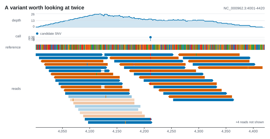
A track owns one horizontal band. It knows how tall it wants to be and how to draw itself, and nothing else: it is never told where it sits or which other tracks share the figure. The figure stacks the bands top to bottom in the order you add them and gives every one the same horizontal scale.

That is what lets you read a figure by running a finger down it: everything the finger crosses is at the same position.

karyon ships 37 track types, and the command line reaches 33 of them. The Gallery sorts them by what you want to show, and the Track catalogue lists each one with its options. A type the crate lacks is one small trait away: see Writing a track.

Tracks that are not laid on the axis

A phylogeny is drawn along its branch lengths rather than along the region, so a plot holding only a TreeTrack or a TanglegramTrack gets no ruler. An IdeogramTrack draws the whole chromosome, because its job is to show where the region is on it, and a SnpTrack spaces its variable sites evenly. Neither gets a ruler on its own either.

Scale

A figure builds one scale and hands it to every track. The scale knows where the region starts, how long it is, and where and how wide the plotting area is, which is all it takes to turn a position into a pixel. Two consequences are worth knowing.

Nothing is clamped. A gene that starts before the window is drawn as the whole shape it is, and the edge of the figure crops it. Clamping would move its start to the border and make it look shorter than it is.

A pixel can cover many bases. Across a genome one pixel may stand for thousands of bases, so a track has to choose what to show for them. Coverage shows the highest value in each pixel by default; the lowest is what keeps a dropout visible:

RustCommand line

.add_coverage(depth)
.adjust(|track| track.aggregate(Aggregate::Min))

--coverage depth.txt --aggregate min

Every decision that changes with zoom, such as when a base is wide enough for its letter, is made in pixels per base, so it means the same at any image width. Scale has the details.

plot() and Figure

plot() is the short way to write a figure: one add_ call per track, in the order they stack, with the region held once and the ruler added at the bottom. The command line is the same builder with spaces instead of dots:

RustCommand line

use karyon::{plot, Aggregate};

plot("chr1:1-1000")?
    .add_coverage(depth)
    .label("depth")
    .adjust(|track| track.aggregate(Aggregate::Min))
    .save("depth.svg")?;

karyon chr1:1-1000 --coverage depth.txt --label depth --aggregate min -o depth.svg

label and adjust reach the track added last, and writing either before a track has been added does not compile.

plot() builds a Figure, the layer underneath, and this draws the same SVG byte for byte:

use karyon::{Aggregate, AxisTrack, CoverageTrack, Figure, Region};

Figure::new(Region::parse("chr1:1-1000")?)
    .push(CoverageTrack::new(0, depth).label("depth").aggregate(Aggregate::Min))
    .push(AxisTrack::new())
    .save_svg("depth.svg")?;

Reach for Figure when a track is built by another constructor, read back before it is drawn, or passed around. A plot hands its figure over with into_figure() and takes a finished track with add_track(), so the two mix freely. A figure's width is a setting, 900 pixels by default; its height is not, because it follows from the tracks and is worked out when the figure is drawn. The Rust API covers both layers.

Genome, Rings and Panels

Some pictures do not fit on one region of one sequence.

Container	Use it for	Start from
Genome	Several sequences end to end, such as the contigs of an assembly, on one axis	Plot::over(genome.region())
Rings	A circular chromosome or plasmid, where position becomes an angle and each layer is a ring	Rings::new(length)
Panels	Several finished drawings on one sheet, lettered in the order you add them	Panels::new().push(&figure, "A")

A Rings plot and a Figure can share one Panels sheet. The recipes show a scan across a whole assembly and a sheet of panels.

Readers

use karyon::{plot, read, Region};

let bed = "chr1\t1000\t1500\tgeneA\t0\t+\n";
let region = Region::parse("chr1:1-2,000")?;
let features = read::interval::features(bed, &region, None)?;

let svg = plot("chr1:1-2,000")?.add_features(features).to_svg();

karyon::read turns BED, bedGraph, GFF3, VCF, SAM, FASTA and the other line-based formats into the values the tracks take, and Tree::parse_newick does the same for a phylogeny. Every reader takes the text as a &str, never a path, so the library opens no files and the same code runs in a shell, in a test and in a web page. The command line uses the same readers.

A file compressed with gzip or bgzip is read as the text inside it, and a BAM is read a window at a time through its index, both with the crate's own decoders, so neither brings in a dependency. CRAM, BCF and bigWig come in through the tool that writes them as text. File formats lists every format, the columns read and the coordinate convention of each.

Coordinates in one paragraph

The region string and the tick labels are 1-based and inclusive, like samtools and IGV, because those are the numbers a person reads. Everything else in the API, such as Feature::new and Variant::new, is 0-based and half-open, like BED, so a VCF position goes in as POS - 1. The readers do that subtraction for you, and Coordinates has the full story.

Where an array starts

add_coverage puts its first value at the left edge of the region. If the array starts somewhere else and the region changes, every value shifts and the figure still looks plausible. Use add_coverage_at(start, values) whenever the array and the region do not start at the same position.

What karyon refuses to draw

Some tracks make a claim rather than just a picture. When the data cannot support the claim, karyon stops with a message instead of drawing something that looks right and is not.

Situation	What karyon does
A tanglegram given one tree	Refuses until --against names the second. One tree drawn against itself has no crossings, which looks like a perfect result.
A homology file whose names match no gene	Refuses and prints the first names that did not match, instead of outlining every gene as having no counterpart.
Identities that could be fractions or percentages	Asks for --identity. A wrong guess turns every ribbon into a perfect match, or every one into the palest shade.
A methylation site that no read covered	Leaves it out and counts it, instead of drawing it as 0% methylated.
A copy number track with no ploidy	Refuses until --ploidy says where balanced sits. A rule in the wrong place swaps every gain for a loss.
A file with nothing in the region	Stops and names the file, instead of drawing an empty lane that reads as a stretch with no data.

All six are the same mistake: a value standing in for the absence of a value.

Why refuse rather than draw something

A figure that is wrong in an obvious way gets questioned. One that is wrong in a plausible way gets published. A tanglegram of one tree, a join that matched nothing and a site that no read covered all draw cleanly, and each of them states a result that nobody measured. An error message costs a minute; a figure like that can cost a conclusion.