Maps
Put samples on a world map or a globe at the coordinates you supply, draw the links your analysis found between them, and wrap a phylogeny around the map.
Library only
There is no map flag on the command line. Everything here is the Rust library.
A map is not a track: longitude cannot share a scale with bases. Map and
PhyloMap are drawings of their own, and they sit beside genomic figures on a
Panels sheet.
Draw locations and explicit links
use karyon::{GeoFlow, GeoLocation, GeoProjection, Map};

let map = Map::new()
    .title("Surveillance sites")
    .subtitle("Counts and coordinates supplied by the analysis")
    .projection(GeoProjection::orthographic(15.0, -5.0))
    .show_labels(true)
    .push(
        GeoLocation::new("Lima", -12.0464, -77.0428)
            .category("South America")
            .count(12),
    )
    .push(
        GeoLocation::new("Madrid", 40.4168, -3.7038)
            .category("Europe")
            .count(16),
    )
    .push_flow(GeoFlow::new("Lima", "Madrid").weight(4.0));

map.save_svg("sites.svg")?;
save_pdf("sites.pdf") writes the same map as PDF, as it does for a
PhyloMap; see How the PDF is made.
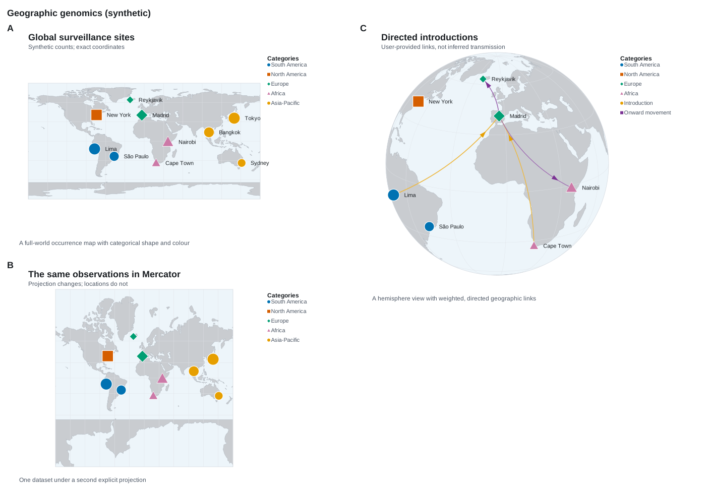
A location's category sets both its colour and its shape, so the legend still
reads without colour. count grows the mark's area with the number of
observations, up to about ten, and the tooltip gives the exact count. value
attaches a number to the tooltip without turning it into a second visual scale.
A flow joins two locations by name. weight thickens its stroke, following the
square root of the weight, and an arrowhead shows its direction; undirected()
drops the arrowhead when the data only support a link. A flow's category
colours it. Nothing here infers a flow: every link on the map is one you pushed.
| Builder | Effect | Default |
|---|---|---|
projection(GeoProjection) |
the map projection, below | Equirectangular |
width(pixels), height(pixels) |
the size of the drawing | 760 by 480 |
margin(pixels) |
whitespace around it | 18 |
push(location), extend(locations) |
add locations, in order | |
push_flow(flow) |
add a link between two named locations | |
show_labels(bool) |
location names beside their marks | off |
show_legend(bool), show_graticule(bool) |
the category key, the latitude and longitude grid | on |
title, subtitle, description |
a heading, a quieter line under it, and the SVG's alt text | |
theme, profile, visual_scale |
colours, a named output profile, the size of text and marks | light theme |
Choose the projection
| Projection | Extent | Behaviour |
|---|---|---|
GeoProjection::Equirectangular |
the whole world, two wide by one high | longitude and latitude evenly spaced; right when area and angle are not the claim |
GeoProjection::Mercator |
the whole world, square | local angles kept; latitude is cut at about 85 degrees rather than sent to infinity |
GeoProjection::orthographic(latitude, longitude) |
one hemisphere, a disc | a globe centred on the given point; what lies on the far side is counted, not drawn |
What a map will not draw
A position must be a finite latitude from -90 to 90 and a longitude from -180
to 180, which is what GeoPosition::is_valid checks. A location outside that
is not clamped into a plausible place: it is left off. A flow whose endpoint
name is missing, shared by two locations or at an invalid position is
unresolved; where two places share a name, karyon does not pick one.
Each of these is counted in a line under the map, as invalid locations,
locations outside the projection, unresolved flows or flows outside the
projection, so a map that drew less than it was given says so.
invalid_location_count() and unresolved_flow_count() return the same
numbers to a pipeline. Tooltips keep coordinates and values to the precision
they were given; only the path geometry is rounded.
Put a phylogeny around the map
use karyon::{GeoLocation, GeoProjection, PhyloMap, Tree};

let tree = Tree::parse(
    "((A[&date=2023.1,country=Peru]:0.2,\
       B[&date=2023.4,country=Peru]:0.3):0.4,\
      C[&date=2023.8,country=Spain]:0.7);",
)?;

PhyloMap::new(tree)
    .title("Circular phylogeography")
    .location_by("country")
    .coordinates([
        GeoLocation::new("Peru", -9.19, -75.0152),
        GeoLocation::new("Spain", 40.4637, -3.7492),
    ])
    .projection(GeoProjection::orthographic(15.0, -18.0))
    .time("date")
    .time_unit("year")
    .save_svg("phylogeography.svg")?;
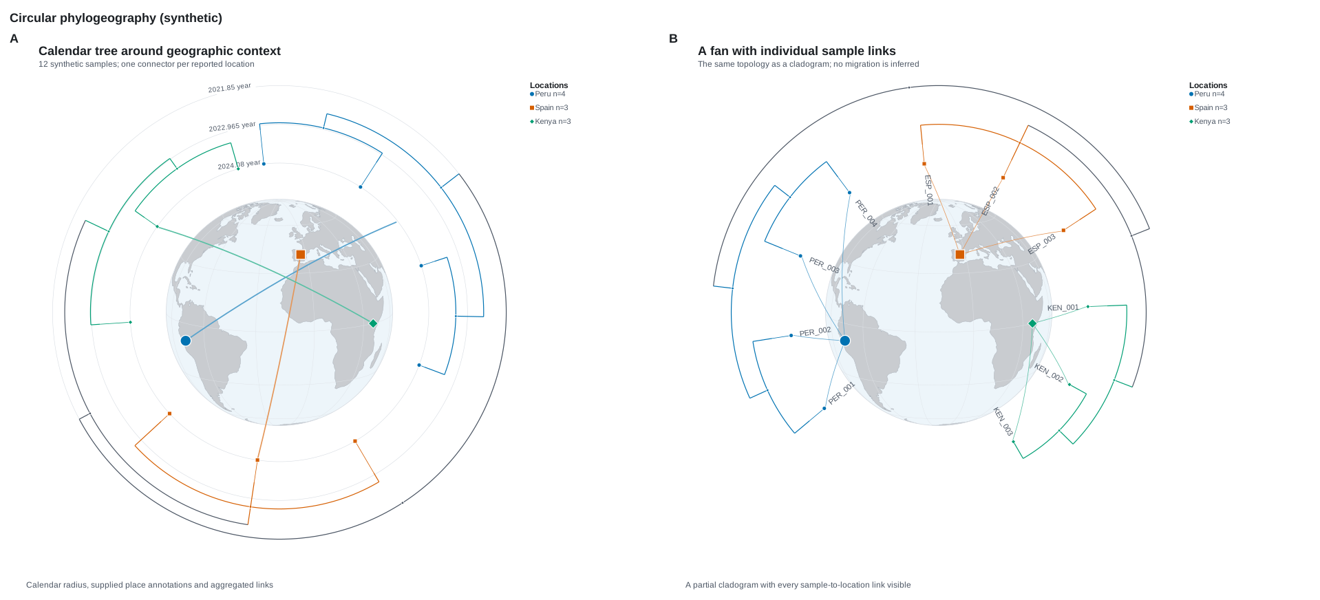
PhyloMap reads one annotation from each tip, joins it by exact name to a
table of coordinates you supply, and draws the tree as a circle around the map.
The tree stays a tree: the map neither changes its topology nor estimates where
its ancestors were.
By default each place gets one connector to the tips that map to it, a little
wider for more tips, with the exact count in its tooltip.
PhyloConnector::Individual draws one named connector per tip, and
PhyloConnector::None keeps only the tree and the marks. All three show the
same table; they are display choices, not different analyses.
| Builder | Effect | Default |
|---|---|---|
location_by(key) |
the tip annotation naming a place, a tip's own or its nearest annotated ancestor's | "location" |
coordinates(places), coordinate(place) |
the named coordinate table; no geocoding or lookup | empty |
projection(GeoProjection) |
the map in the middle | orthographic(15.0, -5.0) |
connector(PhyloConnector) |
Aggregated, Individual or None |
Aggregated |
time(key), time_direction, time_unit |
the radius as a date or height every tip carries | branch length |
shape(TreeShape::Cladogram) |
branches counted rather than measured | Phylogram |
diameter(pixels) |
the size of the tree's circle, at least 320 | 760 |
radial_start(degrees), radial_sweep(degrees) |
rotate the first tip clockwise; sweep 120 to 360 degrees | -95, 350 |
show_tip_labels(bool) |
tip names between the tree and the map | off |
show_time_guides(bool) |
concentric guides when the time layout succeeds | on |
A tip whose place is missing from the table, or named twice in it, or at an
invalid position, is unlocated; a place on the hidden side of the globe is
outside the projection. Both are counted under the drawing and the tip is still
drawn, so missing geography cannot quietly delete a sample. If time cannot
place every tip, the tree falls back to its phylogram or cladogram and the
drawing says the time layout was unavailable.
Branches are coloured only by places already on a node or on an ancestor above
it. karyon does not reconstruct ancestral locations, infer migrations, geocode
names or claim transmission: run that analysis upstream and pass its result as
annotations or as GeoFlow records on a Map.
Compose maps with other drawings
use karyon::{plot, Panels};

let locus = plot("NC_000962.3:761001-763000")?
    .add_coverage(depth)
    .label("depth")
    .into_figure();

Panels::new()
    .columns(2)
    .push_captioned(&locus, "A", "Depth over rpoB")
    .push_captioned(&map, "B", "Where the isolates were sampled")
    .push_captioned(&phylo_map, "C", "Their tree around the same places")
    .save_svg("sheet.svg")?;
Map and PhyloMap implement Drawing, as Figure and Rings do, so any mix
of them goes on one Panels sheet with a letter and a caption each. Each panel
keeps its own coordinates; the sheet only places them.
The land is Natural Earth's 1:110m land data, simplified and compiled into the crate. Natural Earth places its vector data in the public domain. Drawing a map makes no network request, needs no tile server and writes no raster image, and the same input gives the same SVG every time.
Where next
-
Reading trees with their annotations, and drawing them on their own.
-
plot(),Figureand the sheets that hold several drawings. -
Gallery: whole genomes and maps
The maps beside the other whole-view figures.
-
Themes and output profiles, which a map takes as a figure does.