Phylogeny tracks¶

Draw a phylogeny with its metadata and its evidence, two phylogenies against each other, or genomic spans painted onto the clades that carry them.

The Rust snippets use ?, so they belong in a function that returns Result<(), Box<dyn std::error::Error>>. To choose a track by its picture, start from the gallery, and for reading annotated trees, dating them and editing their topology, see Phylogenetics.

TreeTrack¶

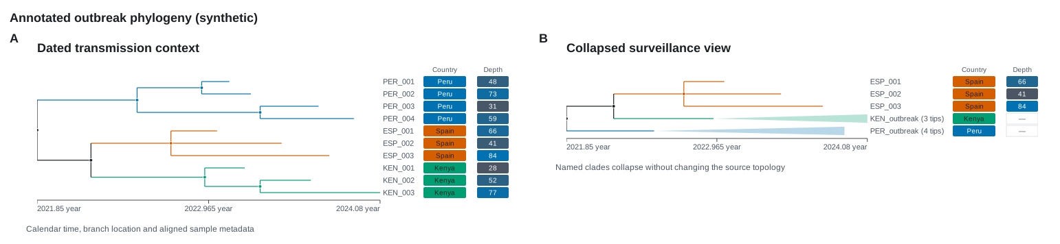
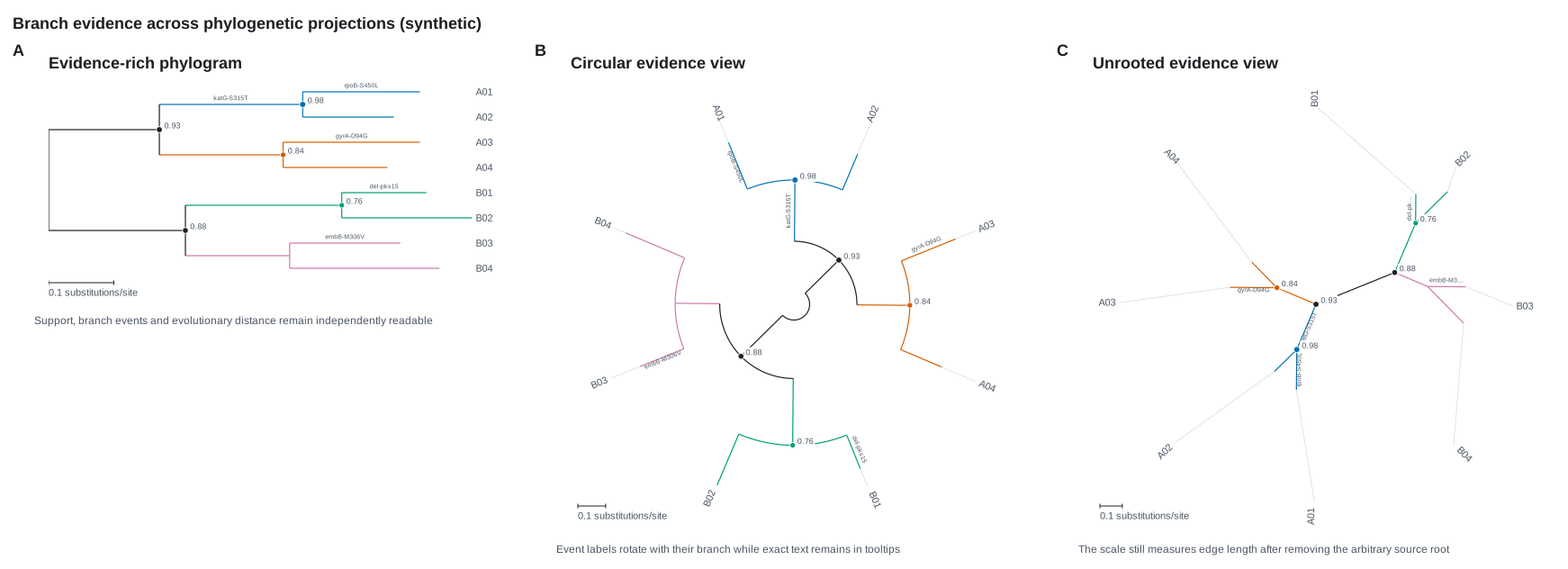
A phylogeny from Newick, drawn as a phylogram when the branch lengths mean something or a cladogram when they do not, in rectangular, circular or unrooted coordinates. Metadata, support, branch events and selection layers go on the same tree.

A synthetic dated outbreak phylogeny with branches coloured by country, aligned country and sequencing-depth columns, and a second view with named clades collapsed


Rust	`.add_tree(tree)` on `plot_tree()`, a plot that names no place, or on `plot()`; `TreeTrack::new(tree)`
Command line	`--tree FILE`, with `--projection`, `--shape`, `--color-by`, `--support-style`, `--threshold`, `--no-scale-bar`, `--mutations`, `--carrying`, `--highlight`, `--focus`, `--max-rows`, `--row-height`, `--traits`, `--columns`
Reads	Newick or NEXUS with BEAST, NHX or IQ-TREE annotations, the first tree of a file of several (`Tree::parse`; `Tree::parse_all` for every one)

RustCommand line

use karyon::{plot_tree, Sheet, SupportStyle, Traits, Tree};

let tree = Tree::parse(
    "((A:0.1,B:0.2)95:0.3,(C:0.2,D:0.1)88:0.2);",
)?;
// sample, lineage and host, one row per tip, as the command line reads it
let sheet = Sheet::parse(&std::fs::read_to_string("samples.tsv")?)?;

plot_tree()
    .add_tree(tree)
    .label("phylogeny")
    .adjust(|track| {
        track
            .traits(Traits::from_sheet(&sheet).strips(["host"]))
            .color_by("lineage")
            .support_style(SupportStyle::Symbols)
    })
    .add_key()
    .save("tree.svg")?;

karyon --tree tree.nwk --traits samples.tsv --columns host \
  --color-by lineage --support-style symbols \
  --label phylogeny -o tree.svg

--traits draws every column of the sheet beside the tips unless --columns names the ones to draw, in the order given; --color-by may name any column of it, drawn or not. A key under the figure names each colour, by its column.

Options¶

Layout and projection

Method	What it does	Default
`.label("phylogeny")`	Names the track in the left gutter (`--label`)	none
`.row_height(18.0)`	Vertical pitch of one tip (`--row-height`)	`15`
`.shape(TreeShape::Cladogram)`	`Phylogram`, with branches as long as their lengths, or `Cladogram`, every branch one step (`--shape`)	`Phylogram`
`.projection(TreeProjection::Circular)`	`Rectangular`, `Circular` or `Unrooted` (`--projection`)	`Rectangular`
`.branch_geometry(BranchGeometry::Curved)`	`Orthogonal`, `Diagonal` or `Curved` branches, in the rectangular projection	`Orthogonal`
`.circular()`	A complete circular tree	off
`.fan(240.0)`	A circular fan sweeping this many degrees	off
`.radial_start(0.0)`	Where a circular tree begins, clockwise degrees from three o'clock	`-90`, twelve o'clock
`.radial_sweep(300.0)`	Clockwise span of a circular tree, in degrees	`360`
`.radial_direction(RadialDirection::Inward)`	Tips towards the circumference, `Outward`, or towards the centre, `Inward`	`Outward`
`.inner_radius(0.2)`	The central gap, as a fraction of the radius	`0.08`
`.radial_size(600.0)`	Requested height of a circular drawing, in pixels	440, larger when the tips need it
`.unrooted()`	An equal-angle tree around a topology-balanced centre	off
`.unrooted_size(600.0)`	Requested height of an unrooted drawing, in pixels	440, larger when the tips need it
`.unrooted_start(0.0)`	Rotates the first equal-angle sector	`-90`
`.max_rows(Some(200))`	Fits the tree in this many rows by collapsing the smallest clades (`--max-rows`)	`None`, no cap
`.collapse(NodeRef::holding("lineage", "L4"))`	Folds one clade into a wedge in the colour of its branches, leaving the tree itself unchanged: an index, a name, or a `NodeRef`; a clade folded by a value is named by it, as `L4 (16 tips)`	none

Rooting

Method	What it does	Default
`.reroot(NodeRef::mrca(["C", "D"]))`	Reroots on an internal node: an index, a name, or a `NodeRef`	the source root
`.reroot_named("L4")`	Reroots on the internal node with this exact name	the source root
`.reroot_outgroup(["B03", "B04"])`	Roots halfway along the edge to a monophyletic outgroup	the source root
`.reroot_midpoint()`	Roots at the midpoint of the longest weighted tip-to-tip path	the source root
`.show_root(false)`	Shows or hides the root diamond in rooted projections	hidden, shown after a reroot

Branches, tips and time

Method	What it does	Default
`.color("#1b1f23")`	Branch colour	from the theme
`.line_width(1.6)`	Branch width	`1.2`
`.show_tips(false)`	Shows or hides the tip names	shown
`.show_nodes(true)`	Draws a point at every visible internal node	off
`.color_by("lineage")`	Colours each branch by an annotation, inherited down the tree (`--color-by`)	none
`.time("date")`	Places the tree on a numeric annotation such as a decimal date	none
`.time_direction(TimeDirection::Decreasing)`	Whether time grows or shrinks from root to tips	`Increasing`
`.time_unit("year")`	What the time axis counts, written as its title: under the numbers of a phylogram, at the inner end of a circle's rings	none
`.support_from("posterior")`	Reads each clade's support from a numeric annotation, as BEAST writes `posterior` and MrBayes `prob` (`--support-from`)	the internal labels
`.show_time_axis(false)`	Shows or hides the time axis that `time` adds	shown

Support, labels and scale

Method	What it does	Default
`.support_style(SupportStyle::Labels)`	Makes support visible: `None`, `Symbols`, `Labels` or `SymbolsAndLabels` (`--support-style none`, `symbols`, `labels` or `both`)	`None`, tooltips only
`.support_threshold(0.8)`	Hides visible support below this, as a fraction or a percentage (`--threshold`)	`0`
`.branch_labels("mutations")`	Writes a branch's own annotation along it, never inherited	none
`.branch_label_size(10.0)`	Font size of those labels	`8`
`.show_scale_bar(false)`	Leaves out the branch-length scale bar a phylogram draws, or with `true` puts it back (`--no-scale-bar`)	drawn on a phylogram with branch lengths
`.scale_bar()`	The same as `.show_scale_bar(true)`	drawn
`.scale_bar_length(0.01)`	An exact scale bar length, in branch-length units	automatic
`.scale_bar_unit("substitutions/site")`	Unit on the scale bar	none

Metadata and decoration

Method	What it does	Default
`.traits(Traits::from_sheet(&sheet).strips(["lineage"]))`	Joins a sample sheet onto the tips by name and draws its columns, widened to fit their headings; the tips it does not name are said under the tree, and `.join()` gives both sides (`--traits`, `--columns`); a column of more values than the palette has colours is drawn as shapes and said to be, and `.colors("lineage", [("L1", "#b78a2c")])` on the sheet gives values colours of their own	none
`.trait_column(TraitColumn::continuous("depth"))`	Adds one metadata column beside the tips, or a ring around them, read from the tree's own annotations	none
`.trait_categorical("country")`	A categorical column, with a stretch of the palette of its own; one with more levels than colours is drawn as symbols	none
`.trait_continuous("depth")`	A continuous column	none
`.trait_bar("depth")`	A bar column, or radial bars	none
`.trait_binary("resistant")`	A presence and absence column	none
`.trait_symbol("host")`	A category shown by colour and shape	none
`.node_glyph(NodeGlyph::pie(["human", "cattle"]))`	A bubble, pie, donut or stacked bar on annotated nodes	none
`.clade_highlight(CladeHighlight::new(NodeRef::mrca(["A", "B"])))`	A translucent field behind one clade, named as `collapse` names one	none
`.highlight_named("L4")`	Highlights the clade with this exact name (`--highlight`)	none

Evolutionary layers

Method	What it does	Default
`.dnds("omega")`	Colours each branch by its own dN/dS on a diverging scale around 1, never inherited	none
`.dnds_label("ω")`	Label of the dN/dS legend	`"dN/dS (ω)"`
`.dnds_neutral_band(0.9, 1.1)`	The ω interval drawn as neutral	`0.95` to `1.05`
`.dnds_saturation(8.0)`	The fold change at which the colour saturates on each side	`4`
`.dnds_significance("q", 0.05)`	Thickens branches whose test annotation is at most this value	none
`.branch_rate_mixture(mixture)`	A weighted capsule of ω rate classes on each branch (`BranchRateMixture`)	none
`.homoplasy_layer(layer)`	Joins branches that carry the same event annotation (`HomoplasyLayer`)	none
`.homoplasy("mutation")`	The same, from an annotation key	none
`.branch_event_layer(layer)`	Ordered event symbols on each branch (`BranchEventLayer`)	none
`.branch_events("mutations")`	The same, from an annotation key	none
`.branch_interval(layer)`	An estimate and interval on each branch (`BranchIntervalLayer`)	none
`.ancestral_states(layer)`	Posterior donuts on internal nodes and marked state changes (`AncestralStateLayer`)	none

Notes¶

What the axes mean. Across, a rectangular tree measures branch length, or time with time, or depth in the tree for a cladogram, so it does not use the figure's shared scale and plot() adds no ruler under it. Its rows are what it shares with its neighbours, because a leaf is a row: a SnpTrack, MatrixTrack, MsaTrack or DomainTrack takes a tree of its own and sorts its rows to match, which is what turns a scatter of shared substitutions into a block.

Projections. circular, fan, radial_start, radial_sweep, radial_direction and inner_radius change the geometry without changing the topology, the branch values or the order of the tips. In circular coordinates time ticks become concentric guides, trait columns become rings and collapsed clades become wedges. branch_geometry changes only the rectangular path of each branch.

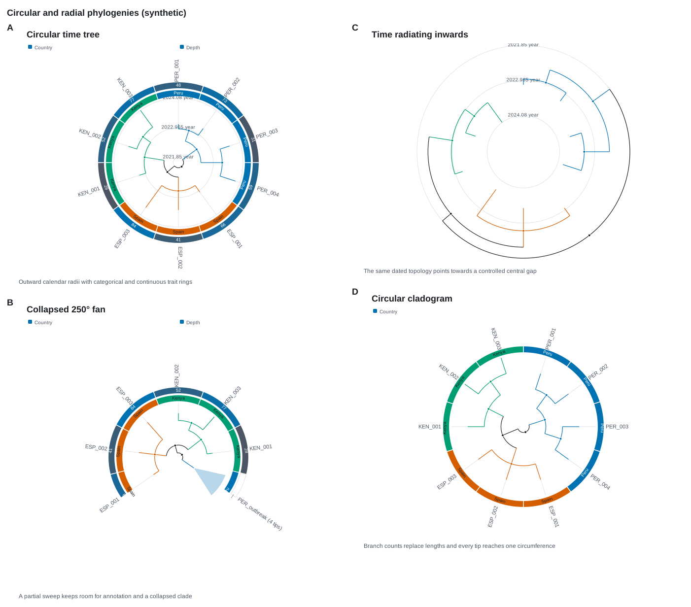
Four radial views of one synthetic outbreak tree: a complete circular time tree with trait rings, a collapsed fan, an inward tree and a circular cladogram

unrooted centres the drawing on a topology-balanced node rather than on the root the Newick happened to write. The bar, binary and symbol columns work in the circular and unrooted projections too, and exact values stay in the tooltips.

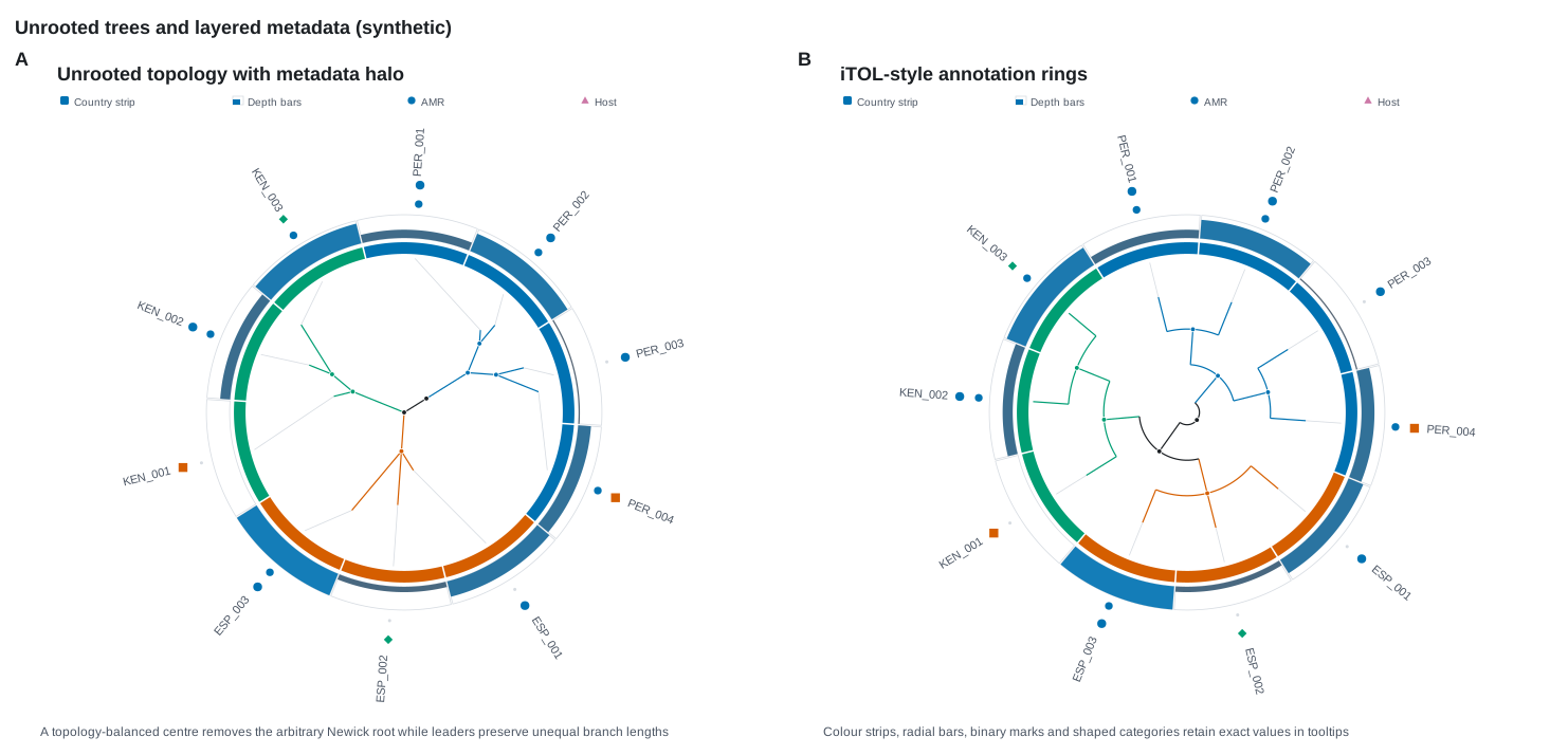
An unrooted phylogram with colour strips, radial depth bars, binary resistance markers and host symbols beside a circular cladogram carrying the same datasets

Metadata. Annotated Newick, BEAST and NHX annotations are kept as typed values on their nodes. time places nodes on a numeric date or height, and every tip must carry it. color_by colours a branch by an annotation inherited down the tree, so a clade whose tips agree takes their colour. On the command line --traits copies a sample sheet onto the tips it names, so the sheet's columns work with --color-by as well as drawing as strips.

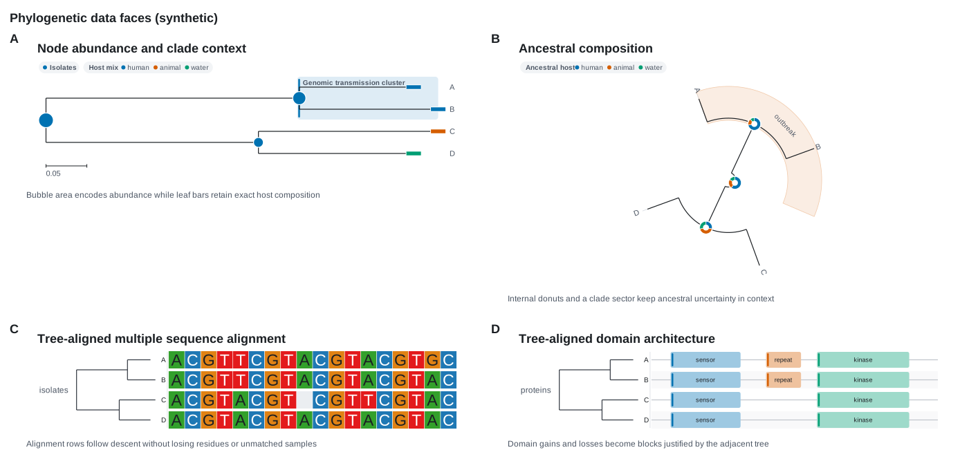
Nodes and clades. NodeGlyph::bubble, pie, donut and stacked_bar attach numbers to nodes; NodeGlyphTarget limits them to internal nodes or leaves, and a missing value draws no glyph rather than a zero. CladeHighlight marks one clade as a band, a sector or a field, depending on the projection, without changing the topology.

A rectangular tree with abundance bubbles and stacked host bars, a radial tree with ancestral-state donuts and a highlighted clade, and tree-aligned genomic rows

Support, labels and scale. support_style makes support visible as scaled symbols, labels or both, and support_threshold takes a fraction or a percentage: 0.8 and 80.0 both mean eighty per cent. A tree's own values are read one way for the whole tree, out of a hundred when any of them runs above one, so a clade at 1 on a bootstrap tree is one per cent. branch_labels prints a node's own annotation along its branch and never inherits an ancestor's, which suits mutations and other events that belong to one branch. scale_bar adds a ruler in branch-length units to a phylogram and refuses to imply those units on a cladogram or a dated tree.

One phylogram in rectangular, circular and unrooted coordinates with support markers and labels, mutation labels and branch-length scale bars

Picking a clade. collapse, reroot and CladeHighlight::new take a NodeRef, and an index or a name is one already. NodeRef::named("L4") is the node with that name, NodeRef::mrca(["S01", "S07"]) the smallest clade holding those tips, as ggtree's MRCA or iTOL's S01|S07 names it, and NodeRef::holding("lineage", "L4") the smallest clade holding every tip whose lineage is L4, read from the sheet traits joined or from the tree's own annotations. A clade found that way that also holds tips it was not named for is still used, and the tips are said under the tree, since a fold over them would say otherwise.

Dates. time reads a number, or a date written as text, as 2020-03-15 or 2020-03, as a decimal year, a month alone at its middle; Tree::time_value gives the value a node is placed at. A BEAST tree gives each node's height, its age back from the most recent tip, and Tree::date_from_height("height", 2021.5, "date") writes each node's calendar date from the most recent tip's, as ggtree's mrsd does, so time("date") draws it against the years. Two tips of one name and a branch of negative length are the file's, drawn as they are and said under the tree.

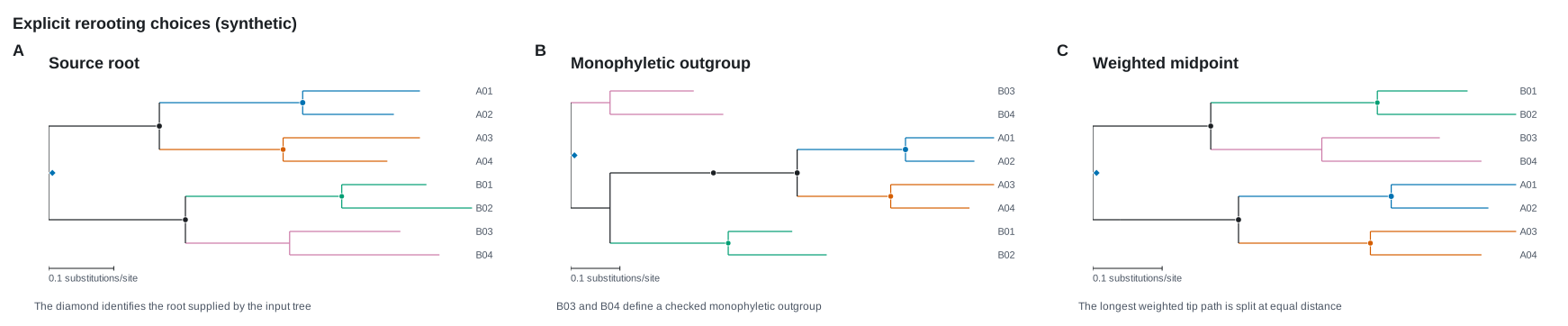
Rooting. The four reroot builders change where the root sits without changing tip-to-tip distances. An outgroup must be monophyletic and the midpoint needs every branch length, and a builder that cannot do what it was asked leaves the tree as it was and says why in a line under the tree, as warnings() does; use Tree::reroot directly when you need to handle that failure. A fold or a highlight asked for before a reroot follows its clade through it. A successful reroot shows a root diamond, which show_root controls, and an unrooted drawing has none by definition.

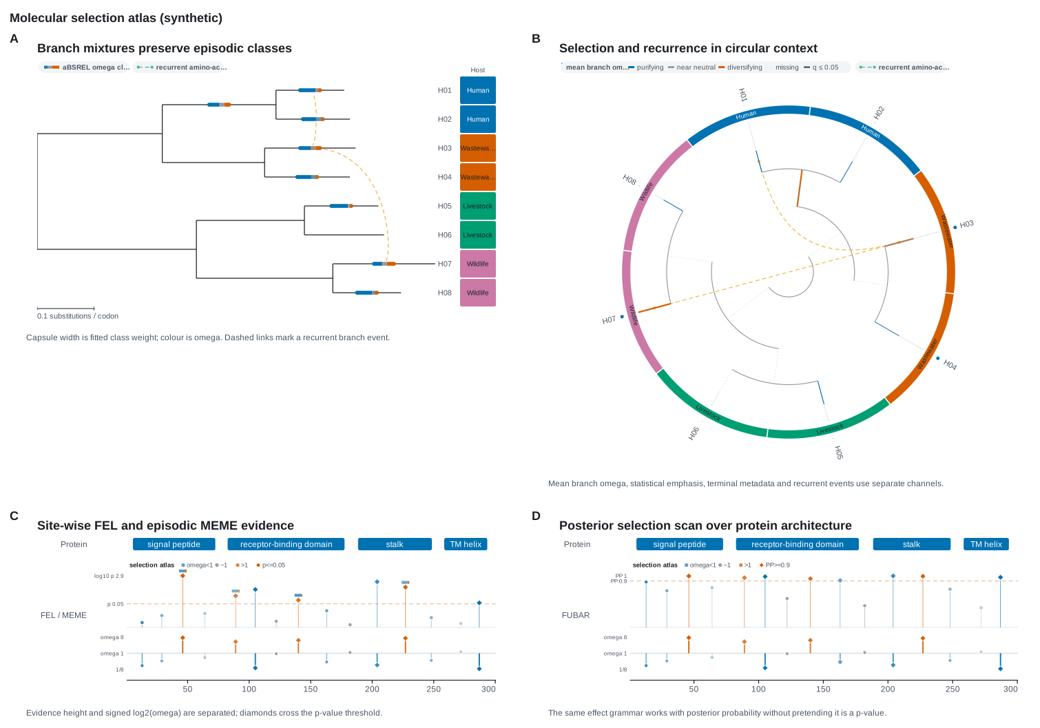
The same phylogram using the source root, a validated monophyletic outgroup and the weighted midpoint, with each root marked by a diamond

Evolutionary layers. dnds colours each branch by its own ω and never inherits a missing one, and dnds_significance changes weight rather than colour, so effect and evidence stay separate. A BranchRateMixture keeps several fitted ω classes on one branch, with capsule width following each class's weight. A HomoplasyLayer joins branches carrying the same event with dashed curves: a picture of recurrence, not a proof of convergence. AncestralStateLayer, BranchEventLayer and BranchIntervalLayer draw state posteriors, ordered events and estimates with intervals, in all three projections. Every layer is keyed across the top of the tree, the dN/dS classes, rate classes, events, intervals, homoplasy and node glyphs each in a chip of their own, and the chips run onto as many rows as they need rather than leaving one out.

A synthetic molecular-selection atlas combining weighted branch rate classes, recurrent-event links, circular mean omega and site scans

Large trees. A tree lays a row per tip and has no cap unless you ask for one. max_rows collapses the smallest clades first until the tree fits, so every tip stays on the figure inside a triangle that says how many it holds; collapse folds one clade by hand, and neither changes the Tree the track owns. From the command line, --focus draws one clade and nothing else, named by its label, by a tip inside it, or by two tips it spans.

TanglegramTrack¶

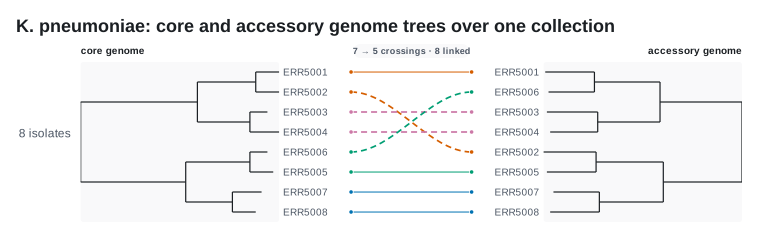
Two trees over the same taxa, drawn facing each other with every shared tip joined across the middle, so their disagreement becomes crossings you can point at. Use it for a gene tree against a species tree, or a core genome tree against an accessory one.

Core and accessory genome trees of eight isolates drawn face to face, the same tips joined across the middle and the crossing ties coloured


Rust	`.add_tanglegram(left, right)` on `plot()`; `TanglegramTrack::new(left, right)`
Command line	`--tanglegram FILE --against FILE`, with `--row-height`
Reads	two Newick or NEXUS files, the left one and the right one (`Tree::parse`)

RustCommand line

use karyon::{plot_tree, TanglegramTrack, Tree};

let core = Tree::parse(
    "((A[&ward=ICU]:0.1,B[&ward=ICU]:0.1):0.2,(C[&ward=Ward]:0.1,D[&ward=Ward]:0.1):0.2);",
)?;
let accessory = Tree::parse(
    "((A[&ward=ICU]:0.1,C[&ward=Ward]:0.1):0.2,(B[&ward=ICU]:0.1,D[&ward=Ward]:0.1):0.2);",
)?;

let track = TanglegramTrack::new(core, accessory)
    .names("core", "accessory")
    .color_by("ward")
    .untangle();
assert!(track.crossings() <= track.initial_crossings());

plot_tree().add_track(track).save("tanglegram.svg")?;

karyon --tanglegram core.nwk --against accessory.nwk -o tanglegram.svg

Options¶

Method	What it does	Default
`.label("isolates")`	Names the track in the left gutter (`--label`)	none
`.names("core", "accessory")`	Names the two trees, drawn over them	none; the command line uses the file names
`.row_height(20.0)`	Vertical pitch of one tip (`--row-height`)	`16`
`.tree_width(0.35)`	Share of the width each tree takes; the rest is the middle	`0.3`
`.shape(TreeShape::Cladogram)`	Phylogram or cladogram, for both trees	`Phylogram`
`.color("#1b1f23")`	Branch colour	theme foreground
`.tie_colors(straight, crossing)`	Colours of a tie that runs straight and one that crosses	from the theme
`.tie_style(TangleTieStyle::Ribbon)`	`Curved`, `Straight` or translucent `Ribbon` ties	`Curved`
`.tie_widths(1.0, 2.0)`	Width of an ordinary and of a crossing tie	`0.9` and `1.5`
`.labels(TangleLabels::Left)`	Where tip names are written: `None`, `Left`, `Right` or `Both`	`Both`
`.label_width(96.0)`	Most room a tip name may take at each side	`72`
`.show_tips(false)`	Shows or hides the tip names down the middle	shown
`.color_by("ward")`	Colours ties by a tip annotation the two trees share	none
`.show_summary(false)`	Shows or hides the crossing and matching summary	shown
`.untangle()`	Rotates clades on both sides to reduce crossings	off
`.untangle_passes(30)`	The same, with a bound on the passes	`12` passes in `untangle`

Notes¶

crossings() is worth a caption, and it is not a statistic. It depends on how each tree happened to rotate its clades, and a clade rotates freely without changing what the tree says. untangle alternates greedy rotations on both sides and keeps only strict improvements, so it never changes a clade or a branch length and never increases the count; it is a deterministic local heuristic, not a global optimum. initial_crossings() and crossing_reduction() report where it started and what it saved, and the summary drawn with the track gives the count before and after, how many tips were joined, and how many only one tree has.

With color_by, each value takes the colour a phylogeny coloured by the same key gives it, in the order the left tree meets the values, and a tie whose two ends disagree about the annotation turns dashed in the foreground ink, which no value is dealt, while each end keeps its own value. legend(&theme) keys the values and the disagreement, and Figure::key() gathers that key.

A tip only one of the trees has is drawn on that tree and joined to nothing, because a taxon missing from one analysis is a fact about the analysis. shared() lists the tips both trees have and unshared() the rest. --against is required: a tanglegram of one tree against itself has no crossings, which is what a perfect result looks like.

CladeTrack¶

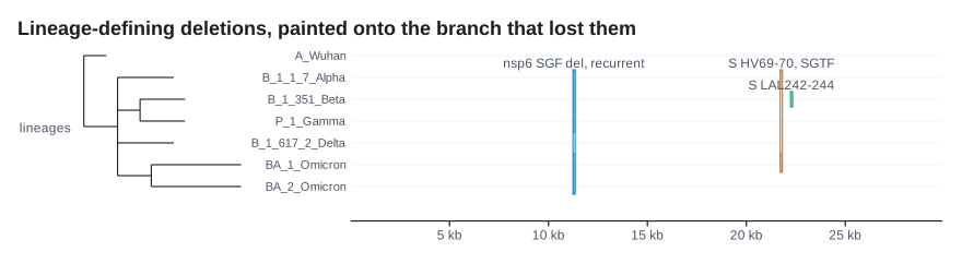
Genomic intervals painted onto a phylogeny: a block whose width is a coordinate span and whose height is the clade that carries it. Use it for deletions, recombinant tracts or acquired islands that were gained or lost on a branch.

Lineage-defining deletions drawn as blocks across a SARS-CoV-2 phylogeny, each spanning the rows of the lineages that carry it, with the recurrent one cut out where a lineage between the carriers does not


Rust	`.add_clades(tree, blocks)` on `plot()`; `CladeTrack::new(tree, blocks)`
Command line	`--clades FILE --with-tree FILE`, with `--row-height`, `--no-names`, `--traits`, `--columns`
Reads	GFF3 with a `taxa` attribute, as `Gubbins` writes it (`read::clade::blocks`), and a Newick tree

RustCommand line

use karyon::{plot, CladeBlock, CladeTrack, Tree};

let tree = Tree::parse_newick("(((A:1,B:1):1,C:2):1,D:3);")?;
let track = CladeTrack::new(
    tree,
    vec![
        CladeBlock::new(1_000, 4_000, ["A", "B"]).name("RD1"),
        CladeBlock::new(6_000, 7_000, ["A", "C"]).name("recurrent"),
    ],
);

assert!(track.is_clade(0));
assert!(!track.is_clade(1));
assert_eq!(track.cut_rows(1), 1);

plot("chr:1-10,000")?.add_track(track.label("lineages")).save("clades.svg")?;

karyon NC_045512.2:1-29,903 --clades gubbins.gff --with-tree tree.nwk --label lineages -o clades.svg

Options¶

Method	What it does	Default
`.label("lineages")`	Names the track in the left gutter (`--label`)	none
`.row_height(16.0)`	Height of one taxon's row (`--row-height`)	`13`
`.row_gap(8.0)`	Gap between rows	`6`
`.tree_width(140.0)`	Room the tree gets, in pixels; `0` hides the tree but keeps its row order	`100`
`.tree_shape(TreeShape::Cladogram)`	Phylogram or cladogram	`Phylogram`
`.show_names(false)`	Shows or hides taxon names between the tree and the blocks (`--no-names`)	shown
`.show_block_names(false)`	Shows or hides block names on blocks wide enough to hold them	shown
`.min_block(3.0)`	Narrowest a block is drawn, in pixels	`2`
`.traits(traits)`	Metadata columns between the names and the blocks (`--traits`, `--columns`)	none

Notes¶

A MatrixTrack cell is one base wide and cells never merge, so a matrix can only say that six samples each carry something here: six observations. A block covering a whole clade says one thing, a single gain or loss on the branch below which every carrier sits. The difference between those two claims is most of what a comparative genomics figure argues about.

The track can lie in only one way, and it refuses to. When the carriers are not every leaf under their common ancestor, the block is still drawn across the rows it spans, but every row inside it that does not carry it is cut out, so a paraphyletic set cannot pass for a clade. is_clade(i) and cut_rows(i) say the same in numbers, for the caption; in the figure above that is a deletion five lineages carry and the lineage sitting between them does not.

The width is a real coordinate span, so the questions a reader asks of a block are coordinate questions: does it cover this gene, do two blocks on different branches share an endpoint. Taxa are joined to leaves by exact name. unmatched() counts the taxa the tree does not have and unplaced() the blocks that therefore could not be drawn, and both counts are printed on the band.

Gubbins writes SEQUENCE in the first column whatever the reference was called, so a file naming one sequence is read as being about the region's sequence, whatever its name. The command line refuses a file whose taxa name no tip of the tree, since a tree with no blocks on it reads as a confident statement that nothing happened.