Read and molecule tracks
Draw the evidence before it became a call: aligned reads, molecules that aligned in pieces, methylation one molecule at a time, splice junctions with their read counts, and raw nanopore current.
The Rust snippets use ?, so they belong in a function that returns Result<(), Box<dyn std::error::Error>>, and names such as reference stand for data you already hold. To choose a track by its picture, start from the gallery.
PileupTrack
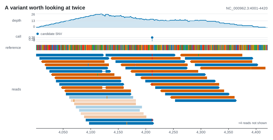
Aligned reads, stacked the way a genome browser stacks them, with the bases that disagree with the reference painted over quiet read bodies. This is the track to open when a variant call looks wrong.
| Rust | .add_pileup(reads) on plot(); PileupTrack::new(reads) |
| Command line | --pileup FILE, with --with-sequence, --fade-by-mapq, --row-height, --max-rows |
| Reads | a BAM, through the .bai beside it where there is one, or SAM text as samtools view writes it (read::bam, read::align::sam) |
use karyon::{read, Plot, ReadColoring, Region};
let region = Region::parse("NC_000962.3:4,001-4,420")?;
let text = std::fs::read_to_string("reads.sam")?;
let reads = read::align::sam(&text, ®ion)?;
// reference: Vec<u8>, the bases from 0-based 4,000
Plot::over(region)
.add_pileup(reads)
.label("reads")
.adjust(|track| {
track
.reference(4_000, reference)
.coloring(ReadColoring::Strand)
.fade_by_quality(true)
})
.save("pileup.svg")?;
Options
| Method | What it does | Default |
|---|---|---|
.label("reads") |
Names the track in the left gutter (--label) |
none |
.reference(4_000, bases) |
The reference from a 0-based start, without which no mismatch can be found (--with-sequence) |
none |
.read_height(10.0) |
Height of one read, in pixels (--row-height) |
9 |
.row_gap(1.0) |
Gap between rows of reads | 2 |
.max_rows(Some(100)) |
Caps the rows drawn; None lifts the cap (--max-rows) |
Some(40) |
.coloring(ReadColoring::Strand) |
What colours a read body: Uniform or Strand |
Uniform |
.color("#b0b7c3") |
Read colour under Uniform |
a wash of the theme's muted ink |
.strand_colors(forward, reverse) |
The two colours under Strand |
the strand colours |
.fade_by_quality(true) |
Fades each read by its mapping quality (--fade-by-mapq) |
off |
.show_mismatches(false) |
Shows or hides mismatched bases | shown |
.mismatch_threshold(0.5) |
Pixels a base needs before mismatches are looked for | 0.2 |
Notes
A read is not an interval, so the track walks its CIGAR. M, = and X all arrive as matches and the track compares the bases itself rather than trusting the letter, while I, D, N, S and H consume what the SAM specification says they consume. That is what puts a mismatch at the right base downstream of an insertion. Without a reference, every read draws as agreeing. A mismatch is painted in its base's colour, and lettered once a base is 7 pixels wide; until then the command line names the four colours in a key under the figure, which Figure::key() gathers in Rust.
Two defaults are refusals. A pileup at thousandfold depth is a thousand rows tall and useful to nobody, so it stops at forty rows and writes +N reads not shown on the band rather than dropping them quietly. And mismatches are only looked for once a base is at least a fifth of a pixel wide, because below that finding one means walking every base of every read to draw something invisible.
A read with mapping quality nought could have come from anywhere, and drawing it as solidly as a uniquely placed one is how a repeat becomes a variant call. With fade_by_quality, reads fade up to full strength at quality 30; a faded read is drawn square, without the arrowhead that says which way it ran, and its mismatches stay at full strength. Reads with no quality stay solid.
Rows are packing, not meaning: reads are sorted by start and dropped into the first row with room, and only the reads on screen are packed. A BAM is read as it is, and only the reads over the window are read where a .bai sits beside it. A CRAM reaches the command line through a pipe, samtools view writing the SAM text this reads from standard input (--pileup -).
The reference is given two ways. --with-sequence FILE, after the pileup, gives it the letters to compare against without drawing them. A FASTA drawn as a track of its own before the pileup, H37Rv.fa --pileup reads.bam, draws the reference row, and the pileup reads against that too, so it is named once.
SplitReadTrack
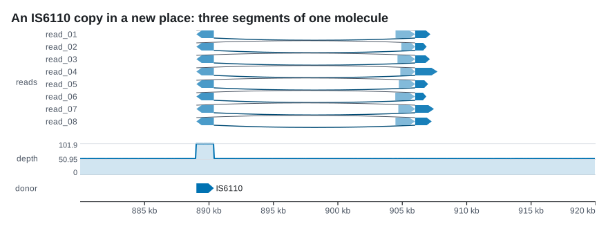
One row per molecule and one bar per alignment, with connectors saying in what order and in which orientation that one piece of DNA visited those places. Use it for the reads behind a structural call.
| Rust | .add_split_reads(reads) on plot(); SplitReadTrack::new(reads) |
| Command line | --split-reads FILE, with --row-height, --no-names |
| Reads | a BAM or SAM carrying SA tags; only primary alignments are read (read::bam, read::split::reads) |
use karyon::{plot, SplitRead, SplitSegment, Strand};

let read = SplitRead::new(vec![
    SplitSegment::new(1_000, 1_600, Strand::Forward),
    SplitSegment::new(9_000, 9_400, Strand::Reverse),
    SplitSegment::new(1_600, 2_100, Strand::Forward),
])
.name("m64011_1");
assert!(read.goes_backwards());

plot("NC_000962.3:1-10,000")?
    .add_split_reads(vec![read])
    .label("molecules")
    .save("split.svg")?;
Options
| Method | What it does | Default |
|---|---|---|
.label("molecules") |
Names the track in the left gutter (--label) |
none |
.row_height(15.0) |
Height of one molecule's bar (--row-height) |
13 |
.row_gap(9.0) |
Gap between rows, where a backward connector runs | 7 |
.min_segment(2.0) |
Narrowest a segment is drawn, in pixels | 3 |
.show_names(false) |
Shows or hides read names (--no-names) |
shown |
.read_ramp(false) |
Whether colour ramps along the read from its 5' end | on |
.color("#0072b2") |
Base colour the ramp is built from | from the theme |
Notes
This is the evidence, and neither neighbour can hold it. A PileupTrack read is one start, one CIGAR and one strand, so a molecule that visits three places cannot be written down in it; a StructuralTrack arc starts from a finished two-breakpoint call, by which point the evidence has been summarised away. A transposition is three segments, not an arc.
A connector that runs backwards is drawn under the row rather than over it, so a read crossing an inversion looks different from one crossing a deletion; goes_backwards() asks the same question in code. The colour ramp from the 5' end is the other half of the claim: it tells a molecule that went A, B, C from one that went C, B, A across the same three places.
SplitRead::new takes segments in read order, and the order is most of what the picture says: sorted by coordinate, the same segments describe a molecule nobody observed. SplitSegment::read_span pins the order to where the bases sat on the read, and the SAM reader works it out from the clipping, measured from the far end for a reverse-strand piece.
Nothing vanishes quietly. A short segment in a wide view is floored at min_segment pixels, and a segment outside the view is counted in the corner of the band.
BisulfiteTrack
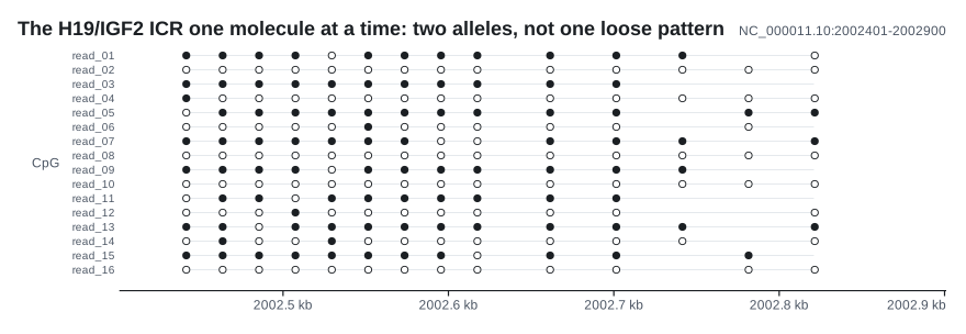
Methylation one molecule at a time: one row per read, one column per site, a filled circle for methylated, a ring for unmethylated, and nothing where the read did not reach. Use it when the question is which molecules are methylated, not how many.
| Rust | .add_bisulfite(sites, molecules) on plot(); BisulfiteTrack::new(sites, molecules) |
| Command line | --bisulfite FILE, with --context, --row-height, --max-rows, --no-names |
| Reads | a bismark_methylation_extractor file (read::bisulfite::molecules) |
use karyon::{plot, Molecule};

let sites = vec![1_010u64, 1_024, 1_031, 1_058];
let molecules = vec![
    Molecule::new("read_1", vec![Some(true), Some(true), Some(true), Some(true)]),
    Molecule::new("read_2", vec![Some(false), Some(false), None, Some(false)]),
];

plot("chr1:1,001-1,100")?
    .add_bisulfite(sites, molecules)
    .label("CpG")
    .save("bisulfite.svg")?;
Options
| Method | What it does | Default |
|---|---|---|
.label("CpG") |
Names the track in the left gutter (--label; the command line uses the context when there is none) |
none |
.row_height(14.0) |
Height of one molecule's row (--row-height) |
12 |
.radius(4.0) |
Radius of one circle | 3.6 |
.color("#1b1f23") |
Colour of the circles | theme foreground |
.show_names(false) |
Shows or hides molecule names (--no-names) |
shown |
.show_rule(false) |
Shows or hides the faint line along each molecule | shown |
.max_rows(Some(100)) |
Caps the molecules drawn; None lifts the cap (--max-rows) |
Some(40) |
Notes
A MethylationTrack gives a fraction per site, and half the reads methylated at every site has two explanations: every molecule methylated at about half its sites, or half the molecules methylated at all of them and half at none. The first is loose modification; the second is two populations of cells or an allele-specific pattern. The site fractions are identical, and one row per molecule tells them apart at a glance: confetti or stripes. discordance() puts a number on it, and site_fraction(i) gives the pooled value back.
The refusal is in the marks. A ring is "measured and not methylated" and no mark is "not measured", two different statements that must not look alike. Columns sit at the real distances between the cytosines, which matters when the question is whether an island is uniformly modified.
A molecule keeps only the sites it covers. Molecule::new(name, calls) takes a call or None for every site, as above; Molecule::covering(name, [(site, methylated)]) takes the covered sites alone, which is what a long read over a few of ten thousand sites wants, and call(site) reads one back. Holding a slot for every site in every molecule made a file of long reads over a wide region cost 708 MB, and the same figure now takes 56.
From an extractor file, both mates of a pair are one row; where they overlap and disagree about a cytosine, neither call is kept. The file's call letter carries the context, and --context picks CpG, CHG or CHH when the file holds more than one.
JunctionTrack
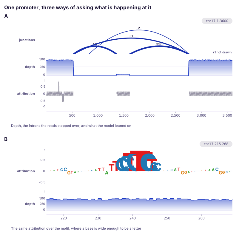
Splice junctions as arcs, each weighted by the reads that crossed it and labelled with the count: the sashimi plot. Stack it over a CoverageTrack so the arcs meet the steps in depth.
| Rust | .add_junctions(junctions) on plot(); JunctionTrack::new(junctions) |
| Command line | --junctions FILE, with --no-counts, --min-reads, --color, --height |
| Reads | an aligner's SJ.out.tab (read::junction::junctions) |
use karyon::{plot, Junction, Motif};

plot("chr1:14,001-17,500")?
    .add_junctions(vec![
        Junction::new(14_829, 14_969, 412).motif(Motif::GtAg),
        Junction::new(14_829, 15_795, 9), // the minor isoform
        Junction::new(15_038, 15_795, 180),
    ])
    .label("junctions")
    .adjust(|track| track.min_reads(3))
    .save("junctions.svg")?;
Options
| Method | What it does | Default |
|---|---|---|
.label("junctions") |
Names the track in the left gutter (--label) |
none |
.height(80.0) |
Band height in pixels (--height) |
64 |
.strokes(1.0, 6.0) |
Thinnest and thickest an arc is drawn | 0.9 to 5.0 |
.saturating_reads(500) |
Reads that make an arc as thick as it gets | 200 |
.min_reads(3) |
Drops junctions crossed by fewer reads, and prints how many (--min-reads) |
1 |
.color("#0072b2") |
Ink of the arcs (--color) |
from the theme |
.show_counts(false) |
Prints or hides the read count over each arc (--no-counts) |
shown |
Notes
A junction nobody crossed is not an observation. It reaches the track, is not drawn, and the band says how many it held back, since a filter nobody can see is worse than no filter. Junction::new is the only way to build one, so a junction always states its read count.
SJ.out.tab counts the intron, 1-based and inclusive, so the start comes back one lower and the end stays. Multi-mapping reads are kept apart and never added to the unique count: a read that mapped in four places would otherwise make a repeat look like an expressed isoform.
Why this is not a structural or split-read track
Three things separate it from a StructuralTrack, which also draws weighted arcs, and none is a setting. An intron sits between two bases, so the feet are at the left edge of a base rather than its middle; at twenty pixels a base that is ten pixels of drift. An intron reaching further is not a bigger event, so height carries nothing: arcs go in lanes so they miss each other, and there is no value axis to invite measuring one. And the ratio between two junctions is the finding, so the count is printed over the apex, with a logarithmic thickness because counts inside one gene span three or four orders of magnitude.
A SplitReadTrack cannot hold the data at all. A spliced alignment is one primary record whose CIGAR steps over the intron, with no SA tag, so read::split::reads counts it as not split. And a split-read track is a row per molecule: four hundred reads over one exon are four hundred rows there and one arc labelled 400 here.
SquiggleTrack
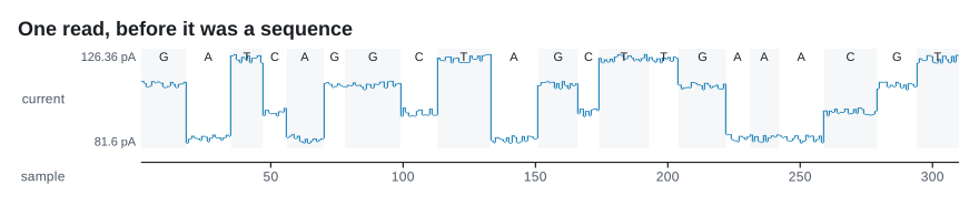
Raw nanopore current for one read, before it was ever a base. When a basecall is in doubt, or a modification is what is being measured, the current is the evidence and the letters are the summary.
| Rust | .add_squiggle(signal) or .add_squiggle_at(start, signal) on plot(); SquiggleTrack::new(start, signal), SquiggleTrack::normalized(start, signal) |
| Command line | --squiggle FILE, or a .slow5 named on its own, with --read, --with-moves for the bases, --color, --height |
| Reads | SLOW5, the text form of BLOW5 that slow5tools view writes, put into picoamperes with each read's digitisation, offset and range; or one sample per number, as picoamperes already (read::series::squiggle). POD5 and FAST5 are binary and are converted first |
use karyon::{plot, Move};

// signal: Vec<f64>, one current sample per entry, in picoamperes
let moves = vec![Move::new(0, b'A'), Move::new(12, b'C'), Move::new(31, b'G')];

plot("read:1-309")?
    .remove_region_label()
    .add_squiggle(signal)
    .label("current")
    .adjust(|track| track.moves(moves))
    .save("squiggle.svg")?;
The figure is laid over the read's samples, counted from 1, so it names no
place; sample:1-500 draws part of it. A file of many reads draws the
first, and says so, unless --read names another. --with-moves
calls.bam puts the bases over it, from the move table Dorado writes with
--emit-moves.
Options
| Method | What it does | Default |
|---|---|---|
.label("current") |
Names the track in the left gutter | none |
.height(120.0) |
Band height in pixels | 90 |
.moves(moves) |
Attaches the basecaller's move table: the first sample of each called base (--with-moves, from SAM or BAM; read::series::moves) |
none |
.color("#0072b2") |
Colour of the trace | theme accent |
.range(60.0, 140.0) |
Pins the current axis | the signal's own range |
.unit(" pA") |
Unit printed after the axis numbers | " pA" |
.show_scale(false) |
Shows or hides the current axis | shown |
.show_bases(false) |
Shows or hides the called bases over the trace | shown |
.point_threshold(6.0) |
Pixels a sample needs before samples are drawn as points | 4 |
Notes
The x axis is sample number, which is time and not position, so the figure goes over a region in samples, as in plot("read:1-309") or Region::new("read", 0, samples), and the locus string printed at the top right says nothing worth keeping.
Above one sample per pixel each column is drawn as the range of the samples under it, the way an oscilloscope or an audio editor draws the same problem: the extremes are honest and the shape between them is not there. Zoom in far enough and the samples are drawn as themselves.
Raw current is comparable within a read and not between reads, since the open-pore current drifts between pores and over the life of a flow cell. SquiggleTrack::normalized subtracts the median and divides by the median absolute deviation, which puts two reads on one axis at the price of an axis in deviations rather than picoamperes; a signal whose deviation is zero is left as it is.
The move table is the only thing in the plot connecting time to sequence. With it, dwells() reports how many samples each called base held the pore, which is the measurement a homopolymer breaks: ten adenines in a row look like one long adenine.