A first program

A figure from Rust: make a project, add the library and write one chain of calls. From the command line, Start here does the same in three steps.

Make a project

Make a new project and add the library:

cargo new first-figure
cd first-figure

[dependencies]
karyon = { git = "https://github.com/PathoGenOmics-Lab/karyon" }

Replace src/main.rs with this whole program:

use karyon::{plot, Aggregate, Feature, Strand, Variant};

fn main() -> std::io::Result<()> {
    // One depth value per base of the region, with a dropout in the middle:
    // the shape a deletion leaves behind.
    let depth: Vec<f64> = (0..2_000)
        .map(|i| if (900..1_030).contains(&i) { 3.0 } else { 55.0 - (i % 23) as f64 })
        .collect();
    let bases: Vec<u8> = b"ACGT".iter().cycle().take(2_000).copied().collect();

    plot("NC_000962.3:761000-762999")?
        .title("rpoB locus, resistance determining region")
        .add_coverage(depth)
        .label("depth")
        .adjust(|track| track.aggregate(Aggregate::Min).height(70.0))
        .add_sequence(bases)
        .label("reference")
        .add_features(vec![
            Feature::new(759_806, 763_325)
                .name("rpoB")
                .strand(Strand::Forward),
            Feature::new(761_081, 761_162)
                .name("RRDR")
                .strand(Strand::Forward)
                .color("#d55e00"),
        ])
        .label("annotation")
        .add_variants(vec![
            Variant::new(761_051).value(0.12).category("synonymous"),
            Variant::new(761_108).value(0.98).category("missense"),
            Variant::new(761_138).value(0.55).category("missense"),
            Variant::new(761_154).value(1.00).category("missense"),
            Variant::new(761_155).value(0.21).category("synonymous"),
        ])
        .label("variants")
        .save("rpoB.svg")?;

    Ok(())
}

cargo run writes rpoB.svg:

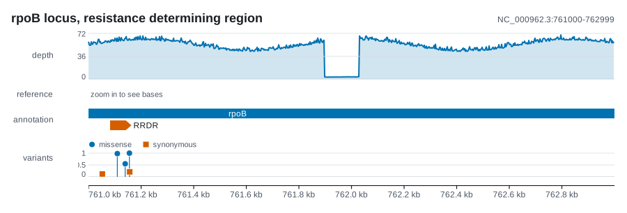
The locus example is this program with seeded, more realistic depth and bases: cargo run --example locus -- assets.

• One call per track, in the order they stack. add_coverage comes first, so depth is on top. Every track gets the same horizontal scale from the figure, which is what keeps them aligned.
• The region is written once. add_coverage and add_sequence lay their arrays from the left edge of the region. When an array starts somewhere else, use add_coverage_at(start, values) or add_sequence_at(start, seq).
• label and adjust apply to the track just added. label names it in the left margin; adjust hands you the track itself to configure. Here it asks for Aggregate::Min, so the dropout survives when several bases share a pixel.
• The ruler is added for you at the bottom. add_axis puts it somewhere else and remove_axis leaves it out.
• A bad region is an error, not a panic. plot reports it as a karyon::Error, which converts into std::io::Error, so one ? covers both the region and the file write.
• to_svg() returns the document as a String instead of writing a file, which is what a web service or a test wants. to_pdf() gives the same figure as PDF, and save writes one when the name ends in .pdf.

Over two thousand bases the reference is too narrow for letters and prints a hint instead. Zooming to base resolution draws the same stack over sixty bases, where every letter shows.

Two coordinate conventions

The region string and the tick labels are 1-based and inclusive, like samtools and IGV. Everything else in the API is 0-based and half-open, like BED. rpoB is 759,807 to 763,325 in the annotation, so it is Feature::new(759_806, 763_325) here, and the call at VCF POS 761,155 is Variant::new(761_154). The file readers subtract the one for you; Coordinates has the full story.

Where to go next

• The Rust API

  Everything plot() and Figure can do.

• Core ideas

  Regions, tracks, the shared scale and what karyon refuses to draw.

• Phylogenetics

  A tree from your files, with its support, your samples beside it, a clade folded, a circle, an alignment in its order or years under it.

• Gallery

  Every kind of figure, with the code that draws it.