Command line

Draw a figure straight from your files without writing any Rust: name a region, then stack one track per file, in the order you want them drawn.

The grammar

karyon <PLACE> [FILE | TRACK FILE]... [OPTIONS]

Four rules cover every command:

1. The place comes first. A region, a gene or a whole sequence:

   • a region is a locus string, 1-based and inclusive as samtools and IGV write it, a sequence name, a colon and a span, with commas and underscores in the numbers ignored, so NC_000962.3:761,000-762,999 and NC_000962.3:761000-762999 are the same 2,000 bases;
   • a gene is a name the figure's annotation gives, and the figure is that gene with a tenth of its length either side, titled with its name;
   • a sequence's name is the whole sequence, which --circular draws as a circle.

   A figure made only of --tree, --tanglegram and --snps tracks takes no place, since none of them is drawn in a window, and neither does a figure across the whole genome: with no place, --manhattan, --coverage, --windows and --copy-number files are drawn over every sequence they name end to end, in the order chromosomes are counted, each as long as the furthest any file reaches on it, or as a bigWig says, and named under the tracks, as karyon tumour.bedgraph tumour.cns --ploidy 2. A sequence a coverage file names no row on is a gap in its track, not a depth of nought, and files that name one sequence draw it as though it were the place written. Anything else needs a place, and one beside them is refused by name: a FASTA, an annotation, calls. So does a scan read with --ld or --with-recombination, or a signal with --format values, and the option is what is named. A BAM or a CRAM, whose depth across a genome is every read it holds, is refused with the mosdepth --by that counts it in windows instead.

   Several places draw one panel each, one under the other, with the same tracks over each, as karyon rpoB katG inhA reads.bam genes.gff3 calls.vcf.gz. A gene is titled with its name and a locus says itself at the top right, the key is drawn once under them all, --title goes over the whole figure, and a track with nothing in one place says so there, as no variants here, where a figure of that place alone is refused. 2. Each file, or each track flag and its file, starts a track. A file named on its own is the kind of track its name says, as the table below has it; a flag in front chooses the kind, as --pileup reads.bam. Tracks stack from top to bottom in the order you write them. 3. The options after a track describe that track, up to the next one. Each is said once per track: a second --label for the same track is refused, since it was almost always meant for the next one. A track given no --label is called after its file. 4. Figure options such as --title and -o belong to no track and can go anywhere on the line.

A file named	Is drawn as
.bam	the depth of its reads (--coverage); --pileup draws the reads
.sam	its reads (--pileup)
.vcf, .bcf	its calls (--variants), a BCF read through its .csi; a cohort's says that --genotypes draws its samples
.gff3, .gff, .gtf, .bed	features (--features); a .bed that is modkit's bedMethyl, as methylation
.bb, .bigbed	features (--features), read through its index
.bedgraph, .bg, .bdg	a signal (--coverage)
.bw, .bigwig	a signal (--coverage), read through its index and its zoom levels
.fa, .fasta, .fna	the reference (--sequence)
.2bit	the reference (--sequence), read through its index
.aln, .afa	an alignment (--msa)
.nwk, .newick, .tree, .treefile	a phylogeny (--tree)
.paf	synteny (--synteny)
.assoc, .glm.linear, .regenie	an association scan (--manhattan)
.cns, .seg	copy number (--copy-number), from CNVkit, or the table IGV and GISTIC2 read; --ploidy is still required
.ld, .bedpe	pairs of positions (--pairs)
.hic	a contact map (--pairs), read through its index at one resolution
.slow5	a read's signal (--squiggle)
a name holding genetic_map	a recombination map (--recombination)

Any of these may end in .gz, except the four read through their index, which are read as they are written and not out of a .gz. A name that could be several things, .tsv or .txt, needs its track's flag, except the genetic maps HapMap and the imputation panels ship, whose names say what they are.

An option and its value may be written as two words or joined by =, as --label depth or --label=depth.

Asking the program

karyon --help fits on one screen: the grammar, every track by what it draws, and the figure options. karyon help coverage, or --help written after a track flag, prints one track's entry and only the options that track takes, with a link to its page here. karyon help all prints everything, every track and every option in full. A flag typed wrong is answered with the one it was probably meant to be:

$ karyon chr1:1-10 --coverge depth.bedgraph
karyon: unknown flag --coverge; did you mean --coverage?

A flag another tool spells, --vcf, --region, --metadata or --legend, is answered with how karyon says the same thing:

$ karyon rpoB --vcf calls.vcf.gz
karyon: unknown flag --vcf; variant calls are --variants FILE, or the VCF named on its own, and --genotypes FILE draws each sample's calls, a row per sample

A worked example

karyon NC_000962.3:761,000-762,999 \
  --coverage depth.bedgraph --label depth --aggregate min --height 70 \
  --sequence H37Rv.fa --label reference \
  --features genes.gff3 --label annotation \
  --variants calls.vcf --label variants \
  --title 'rpoB locus, resistance determining region' -o rpoB.svg

One band per track flag, in the order the flags were written.

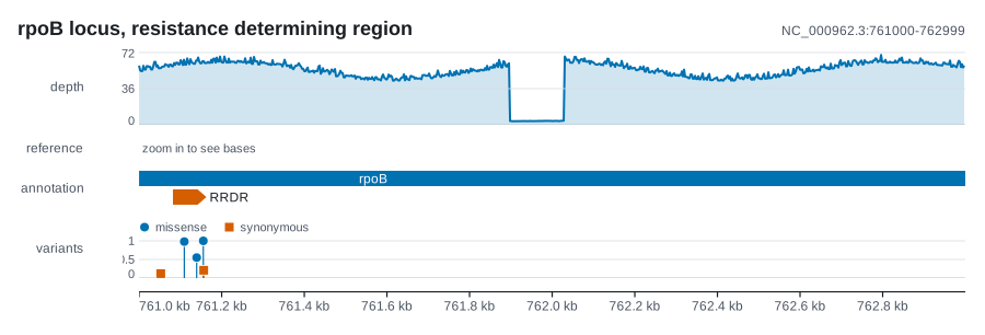
Read the command one flag at a time:

• NC_000962.3:761,000-762,999 is the window every track is drawn over.
• --coverage depth.bedgraph opens the first band. The three options after it belong to it: --label names it in the left gutter, --aggregate min keeps a dropout visible where one pixel covers several bases, and --height sets how tall it is.
• --sequence, --features and --variants open the next three bands, each named by the --label that follows it.
• --title and -o describe the figure, so where they sit does not matter.
• A coordinate ruler is added under the tracks without being asked for.

Every reader skips rows on another sequence and rows outside the window, so you can hand over a genome-wide file and only the window is drawn. The playground runs this same command line in your browser, on example files you can edit.

Spaces instead of dots

The grammar is the plot() builder of the Rust API written with spaces instead of dots. A track flag is an add_ call, and each option after it is a call on that track:

--coverage depth.bedgraph --label depth --aggregate min
.add_coverage(depth).label("depth").adjust(|track| track.aggregate(Aggregate::Min))

The worked example, as Rust:

use karyon::{plot, Aggregate};

plot("NC_000962.3:761,000-762,999")?
    .title("rpoB locus, resistance determining region")
    .add_coverage(depth)
    .label("depth")
    .adjust(|track| track.aggregate(Aggregate::Min).height(70.0))
    .add_sequence(bases)
    .label("reference")
    .add_features(genes)
    .label("annotation")
    .add_variants(calls)
    .label("variants")
    .save("rpoB.svg")?;

The library takes values rather than paths, so depth, bases, genes and calls are already in hand here. Reading them from files is the one thing the command adds, and it does that with the readers in karyon::read, described in File formats.

Track flags

Thirty-seven flags, one per track the command can draw. Each takes one file, or - for standard input, except --axis and --codons, which read nothing.

Flag	Draws	Reads	Track
--coverage <FILE>	per-base signal	bedGraph, bigWig, samtools depth, a bare column of values or a BAM, whose depth it counts	CoverageTrack
--copy-number <FILE>	segmented copy number	a segment table: CNVkit .cns, ASCAT or .seg	CopyNumberTrack
--dynseq <FILE>	per-base model attribution, drawn as the bases themselves	bedGraph or bigWig, with the reference from --with-sequence	DynseqTrack
--junctions <FILE>	splice junctions as arcs weighted by their reads	SJ.out.tab	JunctionTrack
--sequence <FILE>	the reference bases	FASTA or 2bit	SequenceTrack
--features <FILE>	genes and other intervals, a gene drawn once with its exons	BED, GFF3 or GTF, or bigBed	FeatureTrack
--variants <FILE>	point calls	VCF	VariantTrack
--genotypes <FILE>	the call of each sample at each site, a row per sample	VCF with samples	GenotypeTrack
--windows <FILE>	a statistic in windows	bedGraph or bigWig	WindowTrack
--manhattan <FILE>	association statistics	a table of position and value	ManhattanTrack
--recombination <FILE>	recombination rates, as a line in cM/Mb	a genetic map, or a bedGraph of rates	CoverageTrack
--tree <FILE>	a phylogeny	Newick or NEXUS	TreeTrack
--msa <FILE>	a multiple sequence alignment	aligned FASTA	MsaTrack
--snps <FILE>	the variable sites of an alignment	aligned FASTA	SnpTrack
--ideogram <FILE>	cytogenetic bands	a cytoBand table	IdeogramTrack
--matrix <FILE>	a value per sample per site	a matrix table	MatrixTrack
--heatmap <FILE>	a value per sample per window, as a heatmap	a table of windows, as bedtools unionbedg writes it	MatrixTrack
--pileup <FILE>	aligned reads	SAM text from samtools view, or a BAM	PileupTrack
--synteny <FILE>	alignment ribbons between two sequences	PAF from minimap2	SyntenyTrack
--dotplot <FILE>	the same alignments as a dot plot	PAF	DotplotTrack
--orfs <FILE>	open reading frames in six frames	FASTA or 2bit, the file --sequence takes	OrfTrack
--logo <FILE>	a sequence logo	aligned FASTA, the file --msa takes	LogoTrack
--tanglegram <FILE>	two phylogenies face to face	Newick, the left tree; --against names the right	TanglegramTrack
--clades <FILE>	spans carried by named taxa, painted onto a phylogeny	GFF3 with a taxa attribute, as Gubbins writes it; --with-tree names the tree	CladeTrack
--loci <FILE>	gene neighbourhoods from several genomes	BED or GFF3 whose first column names the genome; --links names the homologies	LocusTrack
--methylation <FILE>	modified bases per strand	bedMethyl from modkit	MethylationTrack
--structural <FILE>	structural calls as arcs between their breakpoints	VCF with symbolic alleles or SVTYPE	StructuralTrack
--pairs <FILE>	pairs of places and a value, as a triangle or as arcs	PLINK's .ld, BEDPE or a table of pairs, or a Juicer .hic	PairTrack
--split-reads <FILE>	molecules that aligned in pieces	SAM carrying an SA tag, or a BAM holding them	SplitReadTrack
--bisulfite <FILE>	methylation one molecule at a time	a Bismark methylation extractor file	BisulfiteTrack
--domains <FILE>	protein domains on an axis of residues	an InterProScan table	DomainTrack
--frequencies <FILE>	how often each group was seen at each time	a table of counts over time	SurveillanceTrack
--phylodynamics <FILE>	an estimate over time with its interval	a table of estimates over time	PhylodynamicTrack
--selection <FILE>	a test of selection at each site of a gene	HyPhy's FEL or MEME, or a table of sites	SelectionTrack
--squiggle <FILE>	the current of a nanopore read	SLOW5, or a column of samples	SquiggleTrack
--axis	the coordinate ruler, where the flag sits	nothing	AxisTrack
--codons	a ruler in codons over the coding sequence of the gene the figure is placed on, or of the one gene that codes in the place written, translated where the figure has a --sequence	nothing: the CDS comes from the figure's GFF3, GTF or BED, and the letters from its reference	CodonTrack

--matrix and --heatmap draw one track type from two shapes of table, and --coverage and --recombination another, so thirty-five types are drawn here. The other three are reached from Rust only, and the track catalogue lists all thirty-eight.

A few things about track flags are worth knowing before they surprise you:

• --orfs and --logo work out their track from a file another flag also takes: reading frames from the FASTA --sequence takes, a logo from the alignment --msa takes. Either can sit under the track it was derived from, reading the same file.
• The ruler goes wherever something is measured against it. It is added at the bottom of any figure holding a track laid on the coordinates. --axis puts it where the flag sits instead, and --no-axis leaves the automatic one out. A phylogeny is not laid on the coordinates (its x is branch length), nor is a panel of variable sites (its x is a site index) or an ideogram (its x is the whole chromosome), so a figure of nothing but --tree, --tanglegram, --snps and --ideogram gets no ruler unless you write --axis.
• --codons counts one gene. Placed on a gene by its name, as karyon rpoB genes.gff3 ref.fa --codons, it numbers that gene's CDS; over a place written, as NC_000962.3:761,081-761,200, the CDS of the one gene that codes there, read through the annotation's tabix index where it has one. Codon 1 is the start codon, at the right on the reverse strand, and a trailing partial codon is left off with a note. The CDS has to be one unbroken stretch, in one frame, from its start codon. A gene with no CDS row, two genes in the place or transcripts that code different stretches are refused with what to write instead; a CDS split by introns, one whose rows overlap or meet out of frame, as a ribosomal slippage is written, and one that does not begin on its start codon, by a phase of 1 or 2 or NCBI's start_range, are refused saying why. A ruler over the wrong stretch names the wrong residue at every codon and looks no different. A page that moves the window keeps counting the gene of the place written.
• Some files are their own place. An alignment, a table over time, a table of the sites of a gene and a read's signal need no place named: the figure is drawn over all of it, and its ruler counts columns, weeks, sites or samples rather than bases, numbering them from 1 as the file does. A place narrows it, as week:10-30 or site:50-200. A table whose times have fractions, as a skyline in decimal years has, is a continuous time: its ruler and its tooltips write the times as the file does, to a thousandth, from nought.

• A track flag takes the next word as its file, whatever it is. A forgotten path swallows the flag after it, and the error names the flag it took:

  $ karyon NC_000962.3:761,000-763,000 --coverage --label depth
  karyon: --coverage --label: No such file or directory (os error 2)
  

Track options

Each option describes the track before it. An option given to a track that has no use for it is refused by name rather than ignored, as in --aggregate means nothing to a features track, and where an earlier file takes it, the refusal names that file: it is an option of reads.bam, so write it right after reads.bam. The one exception is --label, which every track takes.

Option	Takes	Applies to	When left out
--label <TEXT>	any text	every track, --axis and --codons included	no name in the gutter; the gene's name for --codons
--against <FILE>	a Newick file, or -	--tanglegram	required
--with-sequence <FILE>	a FASTA or 2bit file, or - for a FASTA	--dynseq, --pileup	required by --dynseq; a pileup reads against the figure's --sequence, and with neither draws every read agreeing
--with-tree <FILE>	a Newick file, or -	--clades, --msa, --snps, --matrix, --heatmap, --genotypes, --domains	required by --clades; for the others the rows stay in the order of their file, and with it they take the order of its tips and the tree is drawn beside them
--links <FILE>	BLAST tabular, or two or three columns of names, or -	--loci	required
--ld <FILE>	PLINK's .ld of the lead against its neighbours, or -	--manhattan	every point in one colour
--with-recombination <FILE>	a genetic map, or -	--manhattan	no rate laid over the scan
--with-moves <FILE>	SAM or BAM as Dorado writes it with --emit-moves, or -	--squiggle	the current alone, with no bases over it
--identity <UNIT>	percent or fraction	--loci	worked out from the values, and refused when they cannot say
--modification <CODE>	m, h, a or another modkit code	--methylation	the one code in the file; refused when it holds several
--context <NAME>	CpG, CHG or CHH	--bisulfite	the one context in the file; refused when it holds several
--analysis <NAME>	Pfam, PANTHER or another member database	--domains	the one analysis in the file; refused when it holds several
--read <NAME>	a read the SLOW5 file names	--squiggle	the first read, and the command says how many the file holds
--resolution <BASES>	a size of bin the .hic holds, in bases, as 10000	--pairs, after a .hic	the finest that cuts the window into 250 bins or fewer, and a note says so where the file holds finer
--ploidy <COPIES>	a number of copies above 0, as in 2	--copy-number	required
--sample <NAME[,N]>	a sample the table names; after --genotypes, samples of the VCF, comma separated, in the order to draw them	--copy-number, --genotypes	the one sample, refused when the table holds several; every sample of the VCF, in the order of its header
--traits <FILE>	a sample sheet, or -	--matrix, --heatmap, --genotypes, --msa, --snps, --clades, --domains, --loci, --tree	no strips
--columns <A,B,C>	column names, comma separated	the tracks --traits applies to, and only with a sheet	every column, in the sheet's order
--height <PX>	pixels	--coverage, --copy-number, --dynseq, --sequence, --variants, --windows, --manhattan, --recombination, --ideogram, --synteny, --dotplot, --methylation, --structural, --pairs, --junctions, --frequencies, --phylodynamics, --selection, --squiggle, --axis	the track's own
--threshold <V|genome-wide>	a number in the file's units, so a p-value for a file of p-values, or genome-wide for -log10(5e-8) on a scan	--manhattan; --tree, as the least support worth showing; --phylodynamics, as a dashed reference; --selection, as the p-value or posterior a site needs; --pairs, as the least value drawn; --frequencies, as the frequency a lineage is flagged at	no line on a scan; every support value on a tree; no reference; p = 0.05, or a posterior of 0.9; every pair; no lineage flagged
--projection <HOW>	rectangular, circular or unrooted	--tree	rectangular
--color-by <KEY>	a column of the --traits sheet, or an annotation in the file	--tree	one colour for every branch
--support-style <HOW>	none, symbols, labels or both	--tree	none: support is in the tooltips only
--support-from <KEY>	an annotation of numbers on the clades, as posterior in a BEAST tree or prob in a MrBayes one	--tree	the internal labels, as a bootstrap writes them
--mutations <KEY>	the annotation the changes are kept under; needs --carrying	--tree	no changes read
--highlight <NAMES>	clade names, comma separated	--tree	nothing highlighted
--carrying <CHANGE>	a change, as the file spells it; needs --mutations	--tree	nothing marked
--shape <HOW>	phylogram or cladogram	--tree	phylogram
--no-scale-bar	nothing	--tree	a scale bar on a phylogram with branch lengths
--focus <NAME[,N]>	a clade label, a tip, or two tips	--tree	the whole tree
--compare-to <NAME>	a row, named as its FASTA header names it	--msa, --snps	the consensus for --msa; the first record for --snps
--no-counts	nothing	--snps, --junctions	counts printed
--min-reads <COUNT>	a whole number of reads	--methylation, --junctions	5 behind a methylation site; 1 across a junction
--fade-by-mapq	nothing	--pileup	every read at full strength
--relative	nothing	--heatmap	the values as they are
--center <V>	a number, as in 0 for a log ratio	--heatmap	one hue from nought up; 1 with --relative
--growth <RISE>	a rise in frequency from one time to the next, above 0 and at most 1, as in 0.15	--frequencies	no rise flagged
--min-total <N>	a whole number of samples from 1	--frequencies	every time drawn
--counts	nothing	--frequencies	frequencies
--row-height <PX>	pixels above 0	--features, --msa, --snps, --matrix, --heatmap, --genotypes, --pileup, --orfs, --tree, --tanglegram, --clades, --split-reads, --bisulfite, --domains	the track's own
--max-rows <N|all>	a number of rows from 1, or all	--pileup, --msa, --snps, --genotypes, --bisulfite, --tree	40 for the first five; no cap on a tree
--no-names	nothing	--features, --msa, --snps, --matrix, --heatmap, --genotypes, --split-reads, --structural, --bisulfite, --domains, --loci, --clades	names drawn
--isoforms	nothing	--features	each gene once, with every exon its transcripts use
--aggregate <HOW>	max, mean or min, which for a bigWig also picks the summary its zoom level is drawn from	--coverage	max
--style <HOW>	area, line or bars for coverage; steps or line for windows; tick or lollipop for variants; differences or all for an alignment; stacked or line for frequencies; triangle or arcs for pairs	--coverage, --windows, --variants, --msa, --frequencies, --pairs	area, steps, lollipop, differences and stacked; for pairs, a triangle where most places were measured against the next one, and linkage and a .hic always
--log	nothing	--coverage, --phylodynamics, --pairs	a linear scale
--max <V>	a number above nought: the top of the scale, as 100 for a depth; for --windows the top, with the bottom as far below the line; for --matrix, --heatmap and --pairs the value drawn at full colour, as 1 for an r²; a heatmap read either side of a centre takes one above it	--coverage, --recombination, --manhattan, --windows, --matrix, --heatmap, --pairs	the largest value in view, rounded up; for windows the furthest either side; for colours the largest value, and 1 for an r²
--color <HEX>	a colour, as in '#d55e00', for the whole track; the values of a --traits column take theirs from the figure option --colors	--coverage, --features, --junctions, --phylodynamics, --squiggle, --pairs, --recombination, --codons	the theme's colours
--genetic-code <N>	an NCBI translation table, 1 to 6, 9 to 16 or 21 to 33, as 2 for vertebrate mitochondria	--codons	the table the CDS names with transl_table=, or 1, whose residues 11 shares; given, it wins, with a note where the CDS names another
--format <NAME>	bedgraph, depth or values for coverage; bed or gff3 for features and loci	--coverage, --features, --loci	told from the file

--height and --row-height never apply to the same track. A track sized by its rows (a feature track, a pileup, an alignment, a tree) takes --row-height and grows with its data, down to a minimum row height of its own. Most other tracks have a fixed height and take --height. --logo and --loci take neither.

Tracks drawn from two files

A track flag takes one path, so the tracks whose data is two files name the second with an option, spelled by what the file is:

Track	First file	Second file
--tanglegram	the left-hand tree	--against, the right-hand tree
--clades	the blocks and the taxa carrying them	--with-tree, the phylogeny they are painted onto
--loci	the genes of each genome	--links, the homologies between neighbouring rows
--dynseq	one score per base	--with-sequence, the reference the letters are drawn from
--pileup	the aligned reads	--with-sequence, optional: the reference mismatches are read against, the figure's --sequence when not given
--manhattan	the scan	--ld, optional: the linkage of each variant with the lead, which colours the points as LocusZoom does; --with-recombination, optional: a genetic map laid over it, read off a scale on the right
--msa, --snps, --matrix, --heatmap, --genotypes, --domains	the rows	--with-tree, optional: the tree the rows are ordered by and drawn beside
--squiggle	the read's current	--with-moves, optional: the basecaller's record of the read, whose move table puts each base over its stretch of current

The first four are refused without their second file:

$ karyon chr1:1-1000 --tanglegram before.nwk
karyon: a tanglegram track is drawn from two files, and --against names the second

Why a missing second file is an error

Each of these tracks would still draw something, and what it drew would look finished and say something false. A tanglegram of one tree against itself has no crossings, which is what a perfect result looks like. A locus track with no homologies outlines every gene as having no counterpart, which reads as a discovery.

A pileup is the one that can do without. It colours the bases that disagree with a reference, and when --with-sequence gives it none it reads against the reference the figure draws:

karyon NC_000962.3:761,000-763,000 \
  --sequence H37Rv.fa --label reference \
  --pileup aln.bam --label reads -o pileup.svg

--with-sequence is for a pileup read against a reference the figure does not draw. With neither, every read is drawn agreeing, since a mismatch is a base that differs from something. A FASTA given to --sequence, --orfs or --with-sequence that holds one record is used whatever its header says; one that holds several is a genome, and the record named like the region's sequence is used, or the command is refused with the names the file does hold.

A tanglegram names its two trees after their files, so the figure says which is which:

karyon --tanglegram before.nwk --against after.nwk --label topology -o tangle.svg

A locus track joins the names in --links to the gene names of the loci file exactly. The names in a search result come from the FASTA it ran against and the names in an annotation from its own columns, and they are often not the same strings. A join that finds nothing is refused, with the first names that failed:

$ karyon locus:1-2,500 --loci loci.bed --links hits.tsv
karyon: --loci hits.tsv: no gene name in this file names anything in the loci, starting with lcl|NC_000962.3_cds_NP_218391.1_3874, lcl|NC_002755.2_cds_MT3978

--identity says whether the third column of the links is a percentage, as BLAST and DIAMOND write it, or a fraction. Left out, a file with any value above 1 is read as percentages, and a file whose values are all at or below 1 is refused, because either reading would draw without failing. The homology table and gene neighbourhoods sections have the columns.

Choosing one of several things in a file

Four formats can hold several datasets in one file: a modkit pileup counting two modifications, a Bismark file with three contexts, an InterProScan table from a dozen member databases, and a segment table with several samples. A file holding one is drawn. A file holding several, with none chosen, is refused with what it holds:

$ karyon NC_000913.3:900-1,100 --methylation dual.bed
karyon: --methylation dual.bed holds h, m, and --modification says which to draw

The option that chooses is --modification, --context, --analysis or --sample. A SLOW5 file holds many reads and is the exception: its first read is drawn, the command says how many others there are, and --read names another. A cohort's VCF is the other: --genotypes draws every sample it names, a row each, and --sample after it chooses the rows and their order rather than one of several, as --sample S07,S01,S12. A name the VCF does not hold is refused with the first five it does. A methylation, bisulfite or domain band is named after what it shows unless --label names it.

--copy-number also needs --ploidy, the copy number that counts as balanced. The segment file does not say it, and a rule in the wrong place turns every gain into a loss.

How deep a stack of rows goes

--pileup, --msa, --snps, --genotypes and --bisulfite stack their data in rows: a pileup packs its reads into rows, and the other four give each sequence, sample or molecule a row of its own. Each stops at 40 rows and prints how many it left out. --max-rows moves the cap, and all removes it:

karyon chr1:1-400 --pileup reads.sam --max-rows 10 --label reads
karyon chr1:1-400 --pileup reads.sam --max-rows all --label reads

A tree has no cap unless you give one, and it answers differently: it folds its smallest clades into triangles until it fits, so every tip is still on the figure inside a triangle that says how many it holds.

karyon --tree big.nwk --max-rows 200 --label phylogeny

The row others are read against

An alignment draws only the cells that disagree with the consensus, and a variable-site panel keeps only the columns where some row disagrees with the first record. --compare-to names the row to compare against instead, spelled as its FASTA header spells it:

karyon aln:1-900 --msa aln.fa --compare-to H37Rv --label alignment

A name the file does not hold is refused with the names it does, and so is a name two records share. --style all draws every cell of an alignment rather than only the disagreements.

Sample sheets beside the rows

--traits takes a sample sheet, joins it to a track's rows by name, and draws one narrow strip per column beside them. --columns picks the columns and their order:

karyon NC_000962.3:1-4,411,532 \
  --matrix genotypes.tsv --label 'resistance alleles' \
  --traits samples.tsv --columns lineage,drug,depth

Nine tracks take a sheet: --matrix, --heatmap, --genotypes, --msa, --snps, --clades, --domains, --loci and --tree. A pileup has rows too, but they are reads, so --traits is refused there. On a tree the strips sit beside the tips, or become rings on a circular or unrooted one, and a folded clade shows what its tips agree on and nothing where they differ. The strips are not placed at coordinates, so they stay put when the region changes.

Two refusals to expect. A sheet whose names match none of the rows is refused with the first names it holds. A column that is not in the sheet is refused with the columns it has:

$ karyon NC_000962.3:1-4,411,532 --matrix genotypes.tsv --traits samples.tsv --columns linage
karyon: --matrix samples.tsv has no column called linage; it has lineage, host, depth, drug

Each column of words starts on a stretch of the palette's six colours of its own. A column of more than six values is drawn in shapes as well, and one that runs past its stretch shares colours with the column after it; a tree says either under it. --colors gives the values colours of your own, the ones your field already knows them by:

karyon tree.nwk --traits samples.tsv --columns lineage,country \
  --colors 'country=China:#1b9e77,India:#d95f02,Kenya:#7570b3,Peru:#e7298a' \
  --colors 'country=Portugal:#66a61e,Spain:#e6ab02,Vietnam:#666666'

The column comes first, then each value and its colour, joined by commas, and the flag again for more values or another column. A colour is # and six hex digits, and quoting the whole word keeps a shell from reading the #. Each pair ends at its colour, so a value may hold a colon, or a comma with no colon before it, as in 'country=Korea, Rep.:#aa0000'. A value not named keeps the palette. The colours are the figure's: every sheet of it that has the column paints those values so, in its strips, in the key and along the branches --color-by colours by the column, drawn as a strip or not. Two values given one colour, or one given the colour the palette deals another, are drawn in shapes as well, and a tree names the two and the colour under it.

A colour that would paint nothing is refused rather than passed over: a --colors with no --traits anywhere, a column no sheet has, a column of numbers (drawn on a ramp), a value no row holds, a column no track draws, and a value given two colours:

$ karyon tree.nwk --traits samples.tsv --colors 'country=Peu:#e7298a'
karyon: --colors names Peu in country, and no row of samples.tsv holds it; country holds China, India, Kenya, Peru, Portugal, Spain, Vietnam

Phylogenies

A --tree track has the most options of any track. A typical figure:

karyon --tree big.nwk --max-rows 60 \
  --traits samples.tsv --color-by lineage --support-style symbols

• --projection lays the tree out as rectangular, circular or unrooted. A circle sizes itself so its tip labels clear each other, up to the width of the figure, so a big tree wants a wider figure or fewer rows.
• --shape cladogram makes every branch one step, the shape to read a topology by when the branch lengths are noise or absent.
• --color-by colours each branch by a column of the --traits sheet or by an annotation the Newick carries. A clade whose tips all agree takes the colour too, so a lineage comes out as a coloured clade. A column of the sheet takes the colours --colors gives it; an annotation of the Newick keeps the palette.
• --support-style makes support values readable without hovering, and --threshold hides the ones below it.
• A phylogram draws a scale bar, a rule in its own branch-length units, and --no-scale-bar leaves it out. It is not the coordinate ruler, which measures the region, and a cladogram or a tree with no branch lengths draws none.
• --focus draws one clade and nothing else, named by its own label, by a tip inside it, or by two tips it spans. A folded triangle gives the pair in its tooltip, and the tree viewer opens a clade the same way.
• --highlight draws a band behind each named clade.

--mutations and --carrying ask who carries a change. An annotated Newick keeps the changes on its branches, under a key the writing tool chose:

(a[&mutations="A123T,S:D614G"]:0.1,b:0.2)[&mutations="C241T"]:0.3;

karyon --tree tree.nwk --mutations mutations --carrying S:D614G

--mutations names the key, and each of the two is refused without the other. A123T, S:D614G, and either with nt: or aa: in front are all read. --carrying then marks everything at or below a branch where that change happened, which is every tip that carries it, and colours by the answer unless --color-by says otherwise. A change that arose twice marks both clades.

A clade, tip, change or --color-by key the tree does not hold is refused with what it does hold, rather than drawing the whole tree:

$ karyon --tree tree.nwk --focus ERR9
karyon: --tree tree.nwk has no tip or clade called ERR9; it has ERR01, ERR02, ERR03

Phylogenetics covers the same tree from Rust, with the layouts and annotations in more depth.

Dense variant calls

A lollipop is a stem with a ringed head, and it reads well up to a few hundred calls. Past that the heads overlap, and every call still costs its share of the file. --style tick draws a plain vertical mark and folds the calls of one colour on one pixel column into a single mark:

karyon chr1:1-4,000,000 --variants calls.vcf --style tick --label variants

A tick does not show the value, so it gives up the height of each call and its tooltip. Colours are kept: two categories on one pixel column are two ticks.

How much smaller

Two hundred thousand calls in four categories over 4 Mb came out at 61 MB as lollipops and 0.28 MB as ticks. A figure 900 pixels wide has fewer than 900 pixel columns to draw in, and ticks draw at most one mark per column and colour.

Telling a file's format

--coverage reads three formats and --features and --loci two each. The format is told from the file (by its column count, a ##gff-version line or its seventh column), and --format overrides the guess where it would be wrong. The words are bedgraph, depth, values, bed and gff3, and Telling formats apart explains each guess.

The case that needs it most is samtools depth over two or more files, which writes four columns, the same count as a bedGraph. karyon notices and says so, and --format depth reads the first sample:

samtools depth -a -r NC_000962.3:761000-763000 sample1.bam sample2.bam \
  | karyon NC_000962.3:761,000-763,000 --coverage - --format depth --label sample1

Figure options

Option	What it does	Default
--title <TEXT>	a title above the stack	no title
--width <PX>	the width of the figure, at most 100,000 pixels	900
--theme <NAME>	light or dark	light
--background <HEX>	the colour under the figure, as #rrggbb, for a page or a slide of another colour; the shades mixed from it follow	the theme's
--no-axis	leaves out the automatic ruler; an --axis track stays	a ruler under the tracks
--no-region-label	leaves out the locus printed at the top right	printed
--no-legend	leaves out the key to the colours of a tree's branches, of --traits strips, and of bases drawn as blocks too narrow for their letters	drawn under the figure
--same-scale	draws the tracks that measure the same thing on one scale, in every panel: the depths of several samples read off one ceiling, so the same height is the same depth. A track given --max keeps its own	each track to its own values
--shade <PLACE[=NAME]>	shades a stretch across every track laid on the coordinates, behind them, named at its head: a locus, one base, a gene, or a span on the figure's own axis; the flag again for another. See Shading a stretch	nothing shaded
--circular	draws the place, one whole sequence, as a circle: each track a ring, the first outermost, inside the ruler, and a key under it naming each ring. --width is the side of the square. See A whole sequence as a circle	along the sequence
--rename <FROM=TO>	reads a sequence a file calls FROM as the figure's TO, as --rename 1=NC_000962.3 for a PLINK table beside a FASTA; several joined by commas, or the flag again	each file's own names
--colors <COLUMN=VALUE:#HEX,...>	colours of your own for the values of a --traits column, as --colors 'country=Peru:#e7298a,Kenya:#7570b3', in its strips, its key and the branches --color-by paints; the flag again for another column. Sample sheets has the rules	the palette, a stretch of it per column
-o, --output <FILE>	writes the figure to a file: PDF when the name ends in .pdf, SVG under any other name	standard output, as SVG
-h, --help	prints the help that fits on a screen, or after a track flag that track's; karyon help all prints all of it
-V, --version	prints the version

-h and -V are answered before anything else on the line is looked at, so karyon --version prints the version whatever else you wrote.

The dark theme is a set of colours chosen for a dark background, not an inversion of the light one:

karyon NC_000962.3:761,000-762,999 \
  --coverage depth.bedgraph --label depth --aggregate min --height 70 \
  --sequence H37Rv.fa --label reference \
  --features genes.gff3 --label annotation \
  --variants calls.vcf --label variants \
  --title 'The same locus, dark theme' --theme dark -o rpoB-dark.svg

Drawn in this page's theme; switch the page to dark with the button at the top to see what `--theme dark` draws.

Shading a stretch

--shade marks a stretch down the whole figure, behind every track laid on the coordinates, as a genome browser marks a region of interest. The place is written as the figure's place is, and a name after = is written at the head of the column:

karyon NC_000962.3:759,001-768,000 reads.bam genes.gff3 \
  --shade NC_000962.3:761,082-761,162=RRDR --shade rpoC -o rpoB.svg

• A span, one base, a gene or a span with no sequence. chr1:1,001-2,000 is a span and chr1:1,500 one base, which marks one column. A gene the annotation names, as --shade katG, is shaded from its own start to its own end, without the margin a figure placed on the gene is drawn with; a gene of --loci where its row draws it, whichever genome its first column names. A span with no sequence, as 120-180, is on whatever axis the figure has: an alignment's columns, a table's weeks or years, said as its ruler says them, or the one sequence it is drawn over.
• Behind the tracks, edged over them. The wash is under every track, so no colour in the figure changes, and its two ends are dashed lines drawn over the tracks, so a heatmap whose cells hide the wash still shows where the stretch starts and stops.
• Only what is on the coordinates. A phylogeny, a tanglegram, a variable-site panel, an ideogram and the key are not, and the column stops at them and goes on under them. Synteny is not shaded either, since its lower bar is the other sequence on a scale of its own.
• Each panel its own. With several places, each panel shades what is on its sequence. A stretch on a sequence no place is on is refused; one on the right sequence and outside the window is drawn as nothing, with a note on standard error, so a figure moved past it is still drawn. A figure across the whole genome is shaded on one of its sequences, as 7:1,001-2,000, by the name the figure or the file gives it, since it reads no annotation to find a gene in.
• Never a file. Many intervals from a BED are what --features draws, and --shade genes.bed is refused with that.

$ karyon chr1:1-1,000 depth.bedgraph --shade chr2:100-200
karyon: --shade chr2:100-200 is on chr2, and the figure is drawn over chr1:1-1,000

Other tools call this highlighting. Here --highlight marks the clades of a --tree, and a place written after it is answered with the --shade that draws it.

A whole sequence as a circle

--circular draws the place round, as circular genome viewers draw a chromosome, a plasmid or an organelle genome: position zero at twelve o'clock, running clockwise, each track a ring in the order written, the first outermost, inside a ruler. The place is one whole sequence, since a circle closes where its sequence ends:

karyon NC_000962.3 --circular genes.gff3 calls.vcf.gz \
  sampleA.bedgraph sampleB.bedgraph --same-scale -o circle.svg

Track	Its ring
--features	an arc a feature, the forward strand on the outer half and the reverse on the inner, as a band of features paints them; named where the ring holds at most 20 named features, and --no-names leaves them off
--coverage	the depth cut into 1,000 arcs, each the --aggregate of its bases (max unless written), read either side of its median: a stretch lost dips inside the line, one carried twice stands outside it
--windows	the windows cut into the same arcs, each the mean of the windows under it, read either side of 0 as the band is
--variants	a tick a call, coloured by consequence in the order the file first names them
--structural	the footprint of each deletion, duplication, inversion and insertion, coloured by class, and a chord across the middle for each breakend join on the sequence
--sequence	the FASTA's GC skew, in windows of a thousandth of the sequence
--axis	the ruler, where it is written; --no-axis leaves it out

• One whole sequence. Named, as NC_000962.3, it is as long as a FASTA, a BAM's header, a VCF's ##contig or a GFF3's ##sequence-region says. A sequence no file gives the length of is refused rather than closed where its last row happens to end, and so is one that two files give different lengths, naming each file and its length, rather than closed at whichever was written first, and so is a gene, which is part of one. A span written from base 1, as NC_000962.3:1-4,411,532, is the whole of a sequence that long, refused where any file says it is another length, which is read from the files' headers and indexes alone, and any other span is part of one. Several places are left for a command each.
• Named in the key and on hover. Each ring is called after its file, or its --label. The ring's name is its tooltip, and the key under the circle gives a line to each ring, outside in, with what its colours mean.
• What a ring takes. --label, --height for its thickness where the track takes one, --aggregate on a depth, --color on a depth or features, --format, and --no-names on features and structural calls. --same-scale puts every ring of depth on one reach, and every ring of windows on another. --title replaces the sequence's name in the middle, and --no-region-label leaves the name and length out.
• What it refuses. A track with no ring is refused by name, a phylogeny with --projection circular, which draws one round. An option a ring would leave unsaid, as --log, --max or --style, is refused rather than passed over, and so is --shade, which has no wedge across the rings.

$ karyon NC_000962.3 --circular reads.bam --log
karyon: --log means nothing to a coverage ring: leave it out, or draw the figure along the sequence, without --circular
$ karyon NC_000962.3:761,000-763,000 --circular genes.gff3
karyon: a circle is a whole sequence, and NC_000962.3:761000-763000 is part of one: name the sequence, as karyon NC_000962.3 --circular, or write the span from 1, as NC_000962.3:1-LENGTH

Standard input

Any file a command names can be -, which reads standard input: a track's own file, and the files named by --against, --with-sequence, --with-tree, --links, --ld and --traits. There is one standard input, so only one of them can take it:

$ karyon NC_000962.3:761,000-763,000 --coverage - --variants -
karyon: only one track can read from standard input

A pipe is read once and kept, so what comes through one is read as a file would be: an alignment, a table over time or over the sites of a gene, and a read's signal are their own place from standard input too, and a table whose times have fractions is read as a continuous time.

The readers drop blank lines, # comment and header lines, and SAM @ headers, so a tool's output pipes in as it comes, with nothing to strip first. Tab and space separated files both read, with the exceptions listed in How a file is read.

Output

The figure goes to standard output unless -o names a file, so it can go into a pipe or a redirect:

karyon Chr1:1-50,000 --manhattan gwas.tsv --label association > scan.svg

-o always names a file: -o - writes a file called -. Leave -o out to write to standard output.

On Windows, name the figure with -o rather than saving it with >. Windows PowerShell 5.1, the one Windows ships, reads what karyon writes through the console's code page and saves it as UTF-16, so the figure on disk is not the bytes karyon wrote: the superscript 2 of an r² comes out as two other characters. cmd, PowerShell 7.4 or newer and Git Bash keep the bytes, and -o writes the same file in all of them.

A name ending in .pdf is written as PDF, from the same drawing:

karyon rpoB reads.bam genes.gff3 calls.vcf.gz -o rpoB.pdf

The page is the figure's size at three quarters of a point to the pixel, the size Inkscape and rsvg-convert give the SVG, so a figure 900 pixels wide is 675 points, about 9.4 inches. Its text is set in Helvetica, Courier and Symbol, which every PDF reader has, rather than in the Inter and JetBrains Mono the SVG asks for, and no font is embedded; the hover titles of the SVG are not carried, since a page has nowhere to hover. A character none of those fonts has, such as a sample name in Cyrillic, is drawn as a question mark, and the command says which on standard error; the figure is still written. How the PDF is made has the rest.

A name that promises any other format, such as fig.png or fig.eps, is refused rather than written as SVG under it, and the message names a tool that writes that format. For a PNG, write fig.pdf and convert it with pdftoppm -png -singlefile -r 300 fig.pdf fig, or fig.svg and convert it with rsvg-convert, Inkscape or a browser; an EPS comes from pdftops -eps, an EMF from Inkscape, and a .svgz from gzip -c fig.svg > fig.svgz.

A journal whose upload checks want every font embedded gets them from Ghostscript, which embeds faces drawn to the same widths:

gs -o embedded.pdf -sDEVICE=pdfwrite -dPDFSETTINGS=/prepress rpoB.pdf

The whole figure is built before any of it is written. A command that fails writes nothing, so a figure left from an earlier run under the same name is not replaced.

Compressed and binary files

A file compressed with gzip or bgzip is read as the text inside it, by every track and from standard input, so a .vcf.gz, a .gff3.gz or a .bed.gz is given as it is.

Through a tabix index

A file compressed with bgzip and indexed by tabix or bcftools index is read a window at a time when its index sits beside it: its header, which is where a VCF names its samples and a table its columns, and the rows over the region, which are all the track draws. A figure of one gene out of a whole genome's calls reads the few blocks over that gene:

tabix -p vcf calls.vcf.gz          # writes calls.vcf.gz.tbi beside it
karyon chr2:5,000,001-5,002,000 calls.vcf.gz -o window.svg

On a VCF of 200 samples and 984,000 rows, 825 MB of text in 82 MB of bgzip, that window took 4.4 seconds and 870 MB read whole, and takes 5 ms and 4 MB through the .tbi. A window of a megabase takes 0.2 seconds. A gene named in a GFF3 beside the calls took 8.9 seconds and 1.3 GB, since the calls were read whole while the gene was looked for and again to draw it, and takes 7 ms: only their header is read while the gene is looked for, for the lengths it states.

The figure is the one the whole file draws, byte for byte, wherever the whole file draws one, since the same rows reach the same reader. Rows outside the region are not read at all, so a row the whole file is refused for, as a VCF line of seven columns, refuses only a region it lies over, and a figure of any other region is drawn. These tracks read through an index, each written as the command beside it writes one:

Track	The file, and its index
--variants, --genotypes	a VCF: tabix -p vcf calls.vcf.gz, or bcftools index calls.vcf.gz for a .csi
--coverage, --windows, --dynseq	a bedGraph: tabix -p bed depth.bedgraph.gz; samtools depth: tabix -s1 -b2 -e2 depth.txt.gz; mosdepth writes its own .csi
--features	a BED: tabix -p bed genes.bed.gz; a GFF3 that says ##gff-version 3, sorted with sort -k1,1 -k4,4n: tabix -p gff genes.gff3.gz
--junctions	an SJ.out.tab: tabix -s1 -b2 -e3 SJ.out.tab.gz
--methylation, with --modification	a bedMethyl: tabix -p bed calls.bed.gz
--manhattan, over a place	an association table: tabix -s1 -b2 -e2 scan.tsv.gz for PLINK 2's #CHROM line or no header, and -S1 with the columns where they are for a plain header line, as -S1 -s1 -b3 -e3 for PLINK 1 once its spaces are tabs
--heatmap	a table of windows with a header: tabix -s1 -b2 -e3 -0 -S1 windows.tsv.gz

PLINK 1 pads its columns with spaces, and tabix splits a row on tabs alone, so it refuses PLINK 1's table as it is written. Turned into tabs first, it indexes:

awk -v OFS='\t' '{$1 = $1; print}' plink.assoc | bgzip > plink.assoc.gz
tabix -S1 -s1 -b3 -e3 plink.assoc.gz

A GFF3 is read over the region and then over as far as the genes over it reach, so a gene whose intron covers the window comes with every exon. The rest are read whole with an index beside them, each for a reason:

• Structural calls: an arc is drawn from the lower of its two breakends, which lies outside a window the arc crosses.
• A recombination map: each rate runs on to the next row, so the rows either side of the window belong to it.
• A GTF, or a GFF3 that does not say it is one: UCSC's GTF holds exon and CDS rows only, so a window inside an intron holds no row of its gene. GENCODE and Ensembl ship the same genes as GFF3, which is read through its index.
• A GFF3 whose exons name a transcript it has no row for, as a GTF turned into GFF3 line by line is written: the transcript reaches from its first exon to its last, and no row says so. The rows the file opens with show it, or the rows over the region; a file that writes its transcripts' rows where it opens and leaves them out further on is drawn through its index without the transcripts that have no exon over the region.
• A bedMethyl with no --modification: the codes it offers to choose from are every code in the file.
• A long table of windows, which names its samples on its rows.

A window a reader refuses sends the file to be read whole, so a row that does not read is refused on its line in the file rather than in the window. A scan with no header is read as p-values when every value it holds lies between 0 and 1, so a window whose values all do is refused that way, and the whole file says what its values are.

The index is looked for where htslib looks for it: calls.vcf.gz.csi, calls.vcf.csi, calls.vcf.gz.tbi, then calls.vcf.tbi, a .csi before a .tbi. Held beside its file in the playground, or by a program through Held, it is read the same way.

An index that does not fit its file is not read: the file is read whole, which draws the same figure, and a note says why, where the file would have been read through a sound index. Beside a GTF, or any other file read whole with its index beside it, the note is left out, since an index written again would leave it read whole:

karyon: calls.vcf.gz.tbi is older than calls.vcf.gz, so it was not trusted and the file was read whole; tabix -f -p vcf calls.vcf.gz writes it again
karyon: calls.vcf.gz.tbi does not describe calls.vcf.gz: the index puts the first row at byte 210, and the file's header ends 240 bytes into the block at byte 0, so the file was read whole; tabix -f -p vcf calls.vcf.gz writes it again
karyon: calls.vcf.gz is compressed with gzip rather than bgzip, so calls.vcf.gz.tbi beside it has no blocks to point to, and the file was read whole; gunzip it, bgzip it and index it again to read it a window at a time

The first is an index last written before its file, counted in whole seconds: it may be the index of an earlier version of the file, and a row that version did not have would be left out of the figure with nothing to show for it. htslib warns of such an index and reads through it anyway. A copy that keeps no times makes an index look older than its file too: cp without -p, rsync without -t, and an archive unpacked without its times. tabix -f writes the index again.

An index named on its own is refused before anything is read, naming the file to give instead:

$ karyon chr1:1-5,000 calls.vcf.gz.tbi
karyon: calls.vcf.gz.tbi is an index, and karyon reads it from beside the file it indexes; name calls.vcf.gz instead

Binary formats

A BAM is read by --coverage, which draws the depth of its reads, and by --pileup and --split-reads, which draw the reads. The index beside it says which blocks hold the reads over the region, so a figure of one gene reads that gene's blocks and no more; without one the file is read from its start. It is looked for where samtools looks for it, a .csi before a .bai: reads.bam.csi, reads.csi, reads.bam.bai, then reads.bai. samtools index -c writes the .csi, which a sequence longer than 536,870,912 bases needs, and a BAM with both is read through the one samtools reads. Depth is counted as samtools depth -a counts it: every base, with reads that are unmapped, secondary, failing quality checks or duplicates left out, and a deletion not counted as covered.

karyon NC_000962.3:761,000-763,000 --coverage aln.bam --pileup aln.bam -o rpoB.svg

A bigWig, a bigBed and a 2bit are read as they are, each through the index it holds, so a window of a whole genome's file reads the few blocks over it. A bigWig is drawn by --coverage, --windows and --dynseq, a bigBed by --features, and a 2bit is the reference to --sequence, --orfs and --with-sequence. Each is told by its first bytes, so one given its track's flag is read whatever it is called. A sequence each one names is a place a figure can be drawn over whole, as a FASTA's or a BAM's is, and a gene a bigBed names is a place too:

karyon chr1:1-2,000,000 signal.bw genes.bb -o signal.svg
karyon geneA genes.bb --sequence genome.2bit -o geneA.svg
karyon chr2 signal.bw -o chr2.svg

Drawn over many bases to a pixel, a bigWig is read from the zoom level of which a pixel holds two bins or more, the coarsest such, rather than from its values as written: a chromosome 900 pixels wide is a few thousand bins of the summary the file keeps for that scale, where its values as written may be millions of spans. Each bin is drawn with what --aggregate takes of a pixel, its most, its least or its mean, with the bases no value covers counted as nought, so the figure is the one the values as written would draw, but for a bin that straddles two columns and is drawn in both: a peak may come out a column wider than it is. Its scale runs to the most of the values under the window, as theirs does, whichever of the three draws the columns. A whole chromosome of 4.7 million spans draws that way in a hundredth of a second and 4 MB. A bigWig written without zoom levels is read as written at any scale.

kent's tools index only the sequences that hold data, so a bigWig or a bigBed written against a whole genome's lengths may name a few of its sequences. Over several places, one on a sequence the file does not name says it has nothing there, as the text the file was written from would; drawn alone, that place is refused naming the sequences the file does have.

A bigBed keeps the columns its header says are BED's own: all twelve of a BED12, so a gene keeps its exons, and the first six of a narrowPeak, whose seventh is a signal value and not where a gene starts coding. A 2bit keeps its runs of N, and its soft-masked runs in lower case, as twoBitToFa writes them.

These three are read out of order, which a pipe cannot be, so each is named rather than piped in; from standard input each is refused with that said. Compressed with gzip, each is refused with the gunzip -k that gives the file back, since its index says where each block is in the file as it is. With no place, a bigWig after --coverage or --windows, or named on its own, is drawn across the whole genome, each sequence as long as its index says and read from the zoom level of which a pixel of the whole genome holds two bins; after --dynseq it needs a place.

A BCF is read by --variants, --genotypes and --structural as the VCF bcftools view prints for it, so each draws from a BCF the figure it draws from the same calls as VCF, byte for byte, and a .bcf named on its own is its calls. The .csi that bcftools index writes beside it, calls.bcf.csi or calls.csi, says which blocks hold the records over the region, so a figure of one gene out of a whole chromosome's calls reads those blocks and no more for --variants and --genotypes; without one, every record is read and those over the region kept. --structural reads every record with an index or without, as it reads a VCF, since an arc is drawn from the lower of its two breakends, which lies outside a window the arc crosses. --variants and --structural read each record's site and pass its samples' columns by undecoded, which are most of a cohort's file, and --genotypes reads each sample's GT and nothing else of them. A cohort's BCF named on its own says how many samples --genotypes would draw, from the names its header gives:

bcftools index calls.bcf           # writes calls.bcf.csi beside it
karyon chr1:100,000,001-100,002,000 calls.bcf --genotypes calls.bcf -o window.svg

Over a chromosome of 248,956,422 bases, a million records of 200 samples, a BCF of 69 MB with its .csi draws a window of 2,000 bases in 10 ms and 6 MB, as the same calls in a VCF of 77 MB of bgzip do through its .tbi, and a megabase of their calls in 27 ms where the VCF takes 36, and of their genotypes in 72 ms where it takes 68. Without an index the BCF takes 2.9 s and 4 MB for that window, where the VCF, 841 MB of text, takes 5.9 s and 851 MB read whole.

The .csi is trusted as a tabix index is: one older than its file, one that does not read as an index, and one that says the file's first record is somewhere other than where its header ends, as the index of another file does, is read past, the file read whole, which draws the same figure, and a note says why:

karyon: calls.bcf.csi is older than calls.bcf, so it was not trusted and the file was read whole; bcftools index -f calls.bcf writes it again

A record a track refuses is named by where it is, the record at chr1:60,000, since a BCF has no lines to number. BCF 2.2 is read, the version htslib reads and bcftools has written since 2014, compressed as bcftools view -Ob writes it, uncompressed as -Ou writes it, or bare.

A .hic is read by --pairs, and named on its own it is drawn as one: the map of the window's sequence with itself, at one of the resolutions the file holds, through the master index at its end and the index of blocks each resolution keeps, so a window reads the few blocks over it whatever the size of the file. --resolution 10000 names the resolution. Without it the finest that cuts the window into 250 bins or fewer is drawn, since a map drawn at its finest over a chromosome is millions of cells and a figure too large to open, and a note says which where the file holds finer:

karyon chr1:20,000,001-22,000,000 contacts.hic --log -o contacts.svg
karyon chr1:20,000,001-22,000,000 --pairs contacts.hic --resolution 5000 --log -o finer.svg

karyon: contacts.hic is drawn at 10,000-base bins, the finest of its 11 resolutions that keeps the window to 250 bins; --resolution 5000 draws finer

Over a chromosome of 248,956,422 bases simulated at 5 kb, 7.6 million cells zoomed out by hictk to eleven resolutions in a .hic of 49 MB, that window of 2 Mb reads 0.5 MB of the file, one block, and draws its 11,370 cells in 0.02 s and 7 MB; the whole chromosome, karyon chr1 contacts.hic, is drawn at 1 Mb in 0.04 s and 12 MB, and the window at 5 kb in 0.04 s and 9 MB. The counts are the raw ones, as hictk prints them with no --balance, and the normalisations a file may carry are not read. Version 9 is read, the version hictk writes; an older file is refused by its version, with the two hictk convert commands, through a .mcool, that write it as version 9.

The .cool and .mcool that cooler writes are HDF5 and are not read, for the reasons File formats gives; each comes in as the BEDPE its tools write, --pairs <(cooler dump --join -r chr1:20000000-22000000 contacts.cool), and a track handed one says so.

CRAM is not read. Hand a track one and it says what the file is and what to write in place of its name:

$ karyon chr1:1-5,000 --pileup aln.cram
karyon: --pileup aln.cram: the file is CRAM, and karyon reads text; write <(samtools view -h aln.cram chr1:1-5000) where its name is, or turn it into text first

<(command) is the shell handing the command's output over as though it were a file, in bash and zsh, so it works for any track and for a second file as well, where - can be given to only one:

karyon NC_000913.3:3,423,000-3,424,000 genes.gff3 \
  --coverage <(samtools depth -a -r NC_000913.3:3423000-3424000 aln.cram) \
  --pileup <(samtools view -h -T ecoli.fa aln.cram NC_000913.3:3423000-3424000) \
  -o reads.svg

A file named on its own, with no flag in front of it, was given its track by its name, and <(command) has no name to give one: on its own it is looked for as a gene or a sequence called /dev/fd/63. So for karyon chr1:1-5,000 aln.cram the message writes the flag in front, write --coverage <(samtools depth -a -r chr1:1-5000 aln.cram) where its name is.

On Windows

cmd and PowerShell have no <(command), and Git Bash's hands over a /dev/fd path that only its own programs can open, not a Windows build of karyon. So the Windows build says to pipe the command in, with - where the file's name was:

$ karyon chr1:1-5,000 --pileup aln.cram
karyon: --pileup aln.cram: the file is CRAM, and karyon reads text; pipe what samtools view -h aln.cram chr1:1-5000 writes into karyon, with - where its name is, or turn it into text first

samtools view -h aln.cram chr1:1-5000 | karyon chr1:1-5,000 --pileup - -o reads.svg

That line runs as it is in all three shells. Only one track can read standard input, so a second file is written to a file of its own first, with the tool's own output option, as samtools view -h -o reads.sam aln.cram chr1:1-5000, and named. Under WSL the Linux build runs, and <(command) works as above.

A file named on its own is answered with its flag in front of the -, as with --coverage - where its name is, since a bare - has no name to say which track reads it.

Secondary and supplementary alignments

--pileup draws every mapped record it is given, secondary and supplementary ones included. Leave them out on the way in with samtools view -F 0x900 if you do not want them.

When something fails

A failing command prints one line to standard error, starting with karyon:, and exits with status 1. Success exits with 0, and so do --help and --version. The first problem stops the command, and nothing is written.

A figure drawn with something its reader should know is still drawn and still exits with 0, and the something goes to standard error, after karyon: too: a sequence no file gives the length of, drawn only as far as its rows reach; a BAM named on its own over a window of reads, drawn as its depth; an index beside a file that was not read, with why and the command that writes it again, as above; and bases too narrow for their letters, with the --width that would letter them. Each is said once, however many panels of a figure of several places it is true of, and the --width said is the one that letters the bases of every panel:

$ karyon NC_000962.3:761,100-761,500 aln.bam H37Rv.fa -o reads.svg
karyon: aln.bam is drawn as its depth; --pileup aln.bam draws its reads
karyon: the bases are blocks of colour at this width, too narrow for their letters; --width 3000 draws the letters

The command line is checked before any file is opened:

$ karyon --features genes.gff3
karyon: the first argument is the place, as in NC_000962.3:761,000-763,000, or a gene or a sequence drawn whole; --coverage, --copy-number, --windows and --manhattan tracks alone are drawn across the whole genome, and a figure of --tree, --msa, --snps, --logo, --tanglegram, --frequencies, --phylodynamics, --selection or --squiggle tracks goes without one

$ karyon trait.assoc genes.gff3
karyon: --features genes.gff3 is drawn over a place, and with none a figure is drawn across the whole genome, which --coverage, --copy-number, --windows and --manhattan tracks alone are: write the place first, as chr1 for a sequence drawn whole or chr1:1-2,000,000 for a stretch of it

$ karyon trait.assoc gwas.assoc --ld lead.ld
karyon: --manhattan gwas.assoc is drawn over a place with --ld, since the linkage to a lead is read over one stretch of one sequence: write the place first, as chr1 for a sequence drawn whole or chr1:1-2,000,000 for a stretch of it

$ karyon reads.bam
karyon: reads.bam is a BAM, which is drawn over a place, as karyon chr1 reads.bam: across a whole genome its depth is every read it holds, so count it in windows with mosdepth --by 100000 sample reads.bam and draw the sample.regions.bed.gz it writes

$ karyon NC_000962.3:0-1000 --coverage depth.bedgraph
karyon: invalid locus "NC_000962.3:0-1000": 1-based coordinates start at 1, not 0

$ karyon NC_000962.3:761,000-763,000 --label depth
karyon: --label describes the track before it, and no track has been given yet

$ karyon NC_000962.3:761,000-763,000 --coverage depth.bedgraph --label depth --label reads
karyon: --label is given twice to one coverage track, which takes one; a flag describes the track written before it

$ karyon NC_000962.3:761,000-763,000 --coverage depth.bedgraph --height NaN
karyon: --height does not take "NaN", only a number of pixels above nought, as in 80

$ karyon NC_000962.3:761,000-763,000 --coverage depth.bedgraph -o rpoB.png
karyon: rpoB.png names a PNG file, and karyon writes SVG and PDF: write rpoB.pdf and convert it with pdftoppm, or rpoB.svg with rsvg-convert, Inkscape or a browser

$ karyon NC_000962.3:761,000-763,000 --coverage depth.bedgraph --aggregate median
karyon: --aggregate does not take "median", only max, mean or min

$ karyon NC_000962.3:761,000-763,000 --coverage depth.bedgraph --style steps
karyon: --style does not take "steps", only area, line or bars for a coverage track

$ karyon NC_000962.3:761,000-763,000 --features genes.gff3 --aggregate min
karyon: --aggregate means nothing to a features track

$ karyon NC_000962.3:761,000-763,000 depth.bedgraph genes.gff3 --aggregate min
karyon: --aggregate means nothing to a features track; it is an option of depth.bedgraph, so write it right after depth.bedgraph

$ karyon chr8:1-1000 --copy-number segments.cns
karyon: --copy-number needs --ploidy, since where balanced sits is not in the file

Then the files, in the order the tracks are stacked. Every message names the flag and the file, and the line number when a line did not say what it should. The line number counts comment and blank lines, so it is the line number in your editor:

$ karyon NC_000962.3:761,000-763,000 --features nowhere.bed
karyon: --features nowhere.bed: No such file or directory (os error 2)

$ karyon chr1:1-1000 --features broken.bed
karyon: --features broken.bed: line 2: end is not a number: "three-hundred-and-fifty"

$ karyon 1:1-5,000 --variants calls.vcf
karyon: --variants calls.vcf: no variants in 1:1-5000, though the file holds 12 on chr1

$ karyon aln:1-9 --msa aln.fa
karyon: --msa aln.fa: line 3: an alignment has every record the same length, and "sample_02" is 1 shorter than "sample_01", which is 9 columns

A file that parsed and held nothing for the window is an error too, because an empty band is almost always a wrong region or a wrong sequence name rather than a fact worth drawing. The message takes one of two shapes, the second when the file held records and none of them reached the window:

$ karyon chr7:1-1000 --features genes.gff3
karyon: --features genes.gff3: no features in the region

$ karyon NC_011900.1:5,000-9,000 --clades gubbins.gff --with-tree tree.nwk
karyon: --clades gubbins.gff: no clade blocks in NC_011900.1:5000-9000, though the file holds 1 on SEQUENCE

Check the sequence name first. It has to match the region's exactly: chr1, 1 and NC_000001.11 are three different sequences to every reader.

A codon ruler is refused where the annotation does not give it one unbroken coding sequence to count, saying why, and what to write instead where something can be:

$ karyon NC_000962.3:763,301-763,400 genes.gff3 --codons
karyon: rpoB and rpoC code in NC_000962.3:763301-763400, and --codons counts the codons of one gene: place the figure on one of them by its name, as karyon rpoB in place of NC_000962.3:763301-763400

$ karyon chr1:2,001-2,100 genes.gtf --codons
karyon: abcA codes in 3 pieces with introns between them, and --codons counts one unbroken coding sequence: across the introns it would number bases that are never translated

A circle is refused where nothing says where it closes, where the files disagree on where, or where its place is part of a sequence:

$ karyon NC_000962.3 --circular sampleA.bedgraph
karyon: a circle closes where NC_000962.3 ends, and no file says where that is, only that sampleA.bedgraph reaches 4,411,532: add its FASTA, a BAM, a VCF with ##contig or a GFF3 with ##sequence-region, or write the span from 1, as NC_000962.3:1-LENGTH

$ karyon NC_000962.3 --circular ref.fa other.vcf
karyon: a circle closes where NC_000962.3 ends, and the files disagree on where that is: ref.fa says 4,411,532 bases and other.vcf says 4,411,529 bases; draw it from files that agree on how long NC_000962.3 is

$ karyon rpoB --circular genes.gff3 calls.vcf.gz
karyon: rpoB is a gene, and a circle is a whole sequence: name the sequence it is on, as karyon NC_000962.3 --circular

Where next

• File formats

  What each reader takes from a file, column by column, and where its coordinates land.

• Recipes

  Whole pipelines that end in one of these commands.

• The Rust API

  The same figures built with the plot() builder.

• Track catalogue

  Every track type, including the ones only Rust can reach.