Performance Benchmarks
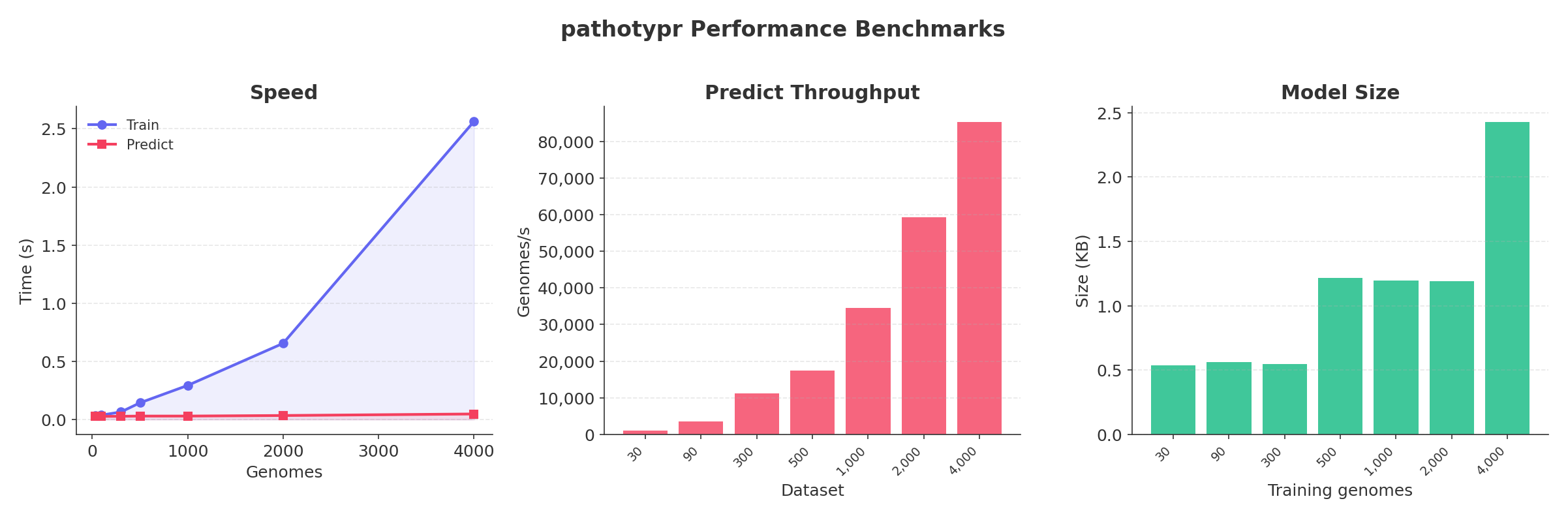
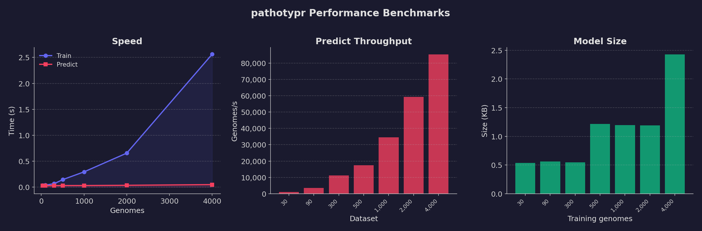
Synthetic benchmarks measuring training and prediction speed, throughput, model size, and memory usage across different dataset sizes. All benchmarks run on a Mac mini M4 (4 threads, k=11, 1000 bp synthetic sequences).
Reproduce these benchmarks:
bash benchmarks/run_benchmarks.sh && python3 benchmarks/plot_benchmarks.py
Dashboard
Training & Prediction Speed
| Genomes | Train time | Predict time | Predict speedup vs train |
|---|---|---|---|
| 30 | 0.032 s | 0.027 s | — |
| 90 | 0.037 s | 0.026 s | — |
| 300 | 0.064 s | 0.027 s | 2.4× |
| 500 | 0.143 s | 0.029 s | 4.9× |
| 1,000 | 0.293 s | 0.029 s | 10.1× |
| 2,000 | 0.654 s | 0.034 s | 19.2× |
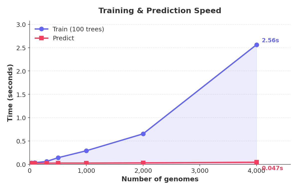
| 4,000 | 2.563 s | 0.047 s | 54.5× |
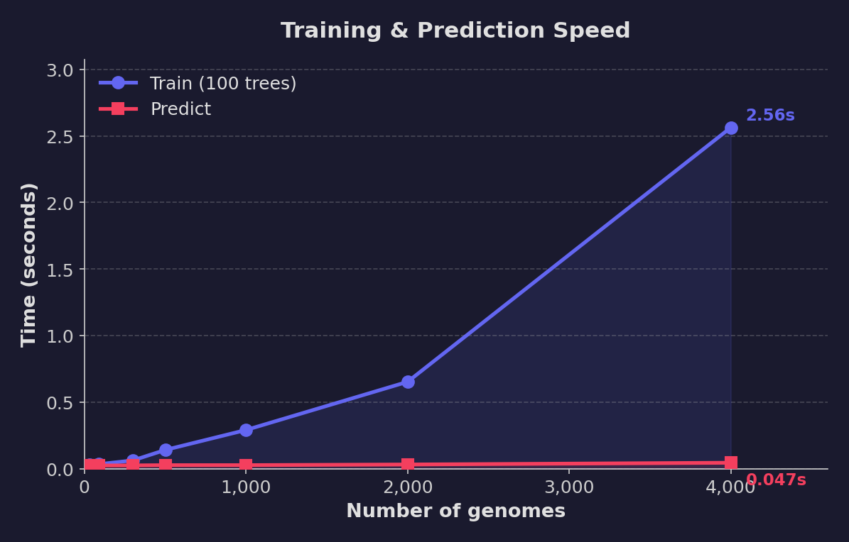
Training scales with dataset size (vectorization + 100 trees). Prediction is nearly constant — streaming batch processing keeps it under 50 ms regardless of input size.
Throughput
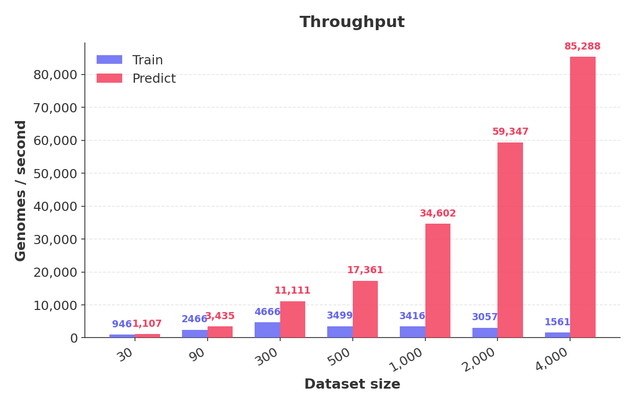
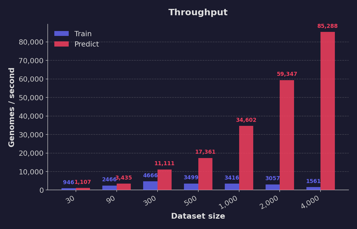
Prediction throughput reaches 85,000+ genomes/second at scale. Training throughput remains above 1,500 genomes/second even at 4,000 samples.
Model Size
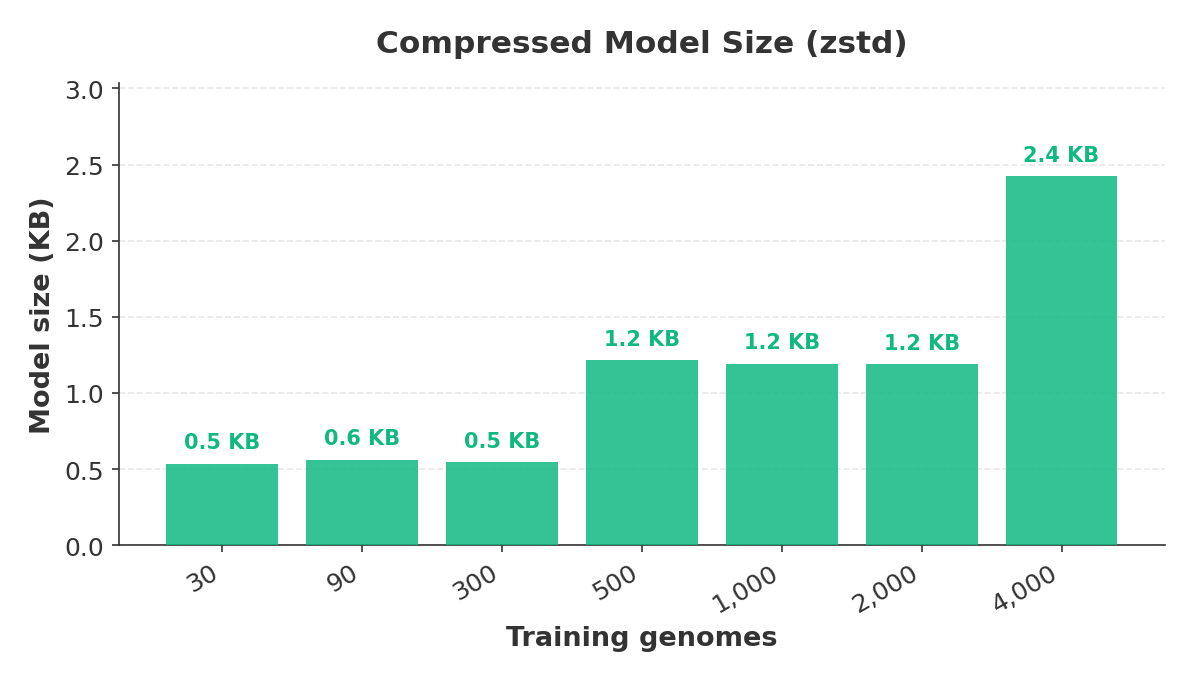
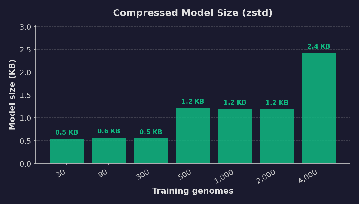
Models are compressed with zstd and stay remarkably small — under 3 KB for all test configurations. Real-world models with full bacterial genomes (4–6 Mb) stay small too — 13–35 KB for the 10- and 50-genome MTB models measured below.
Peak Memory
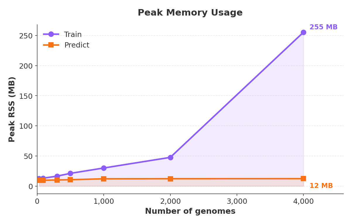
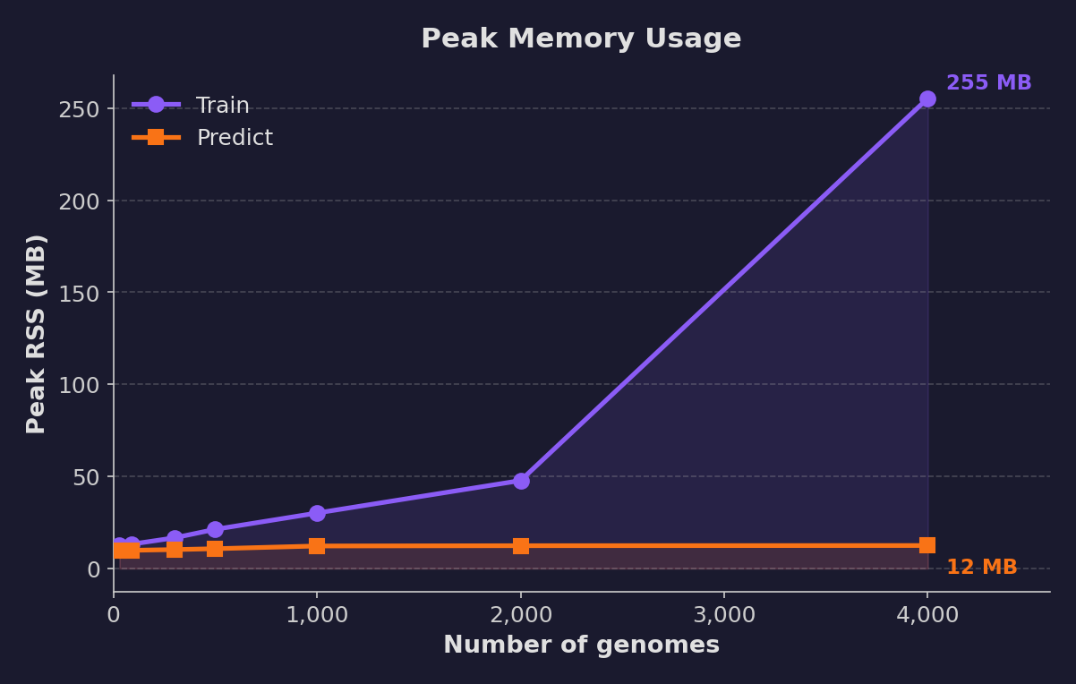
Memory usage grows linearly with training data but remains modest. Prediction memory is dominated by the model size and stays nearly flat.
All Modules — Real M. tuberculosis Data
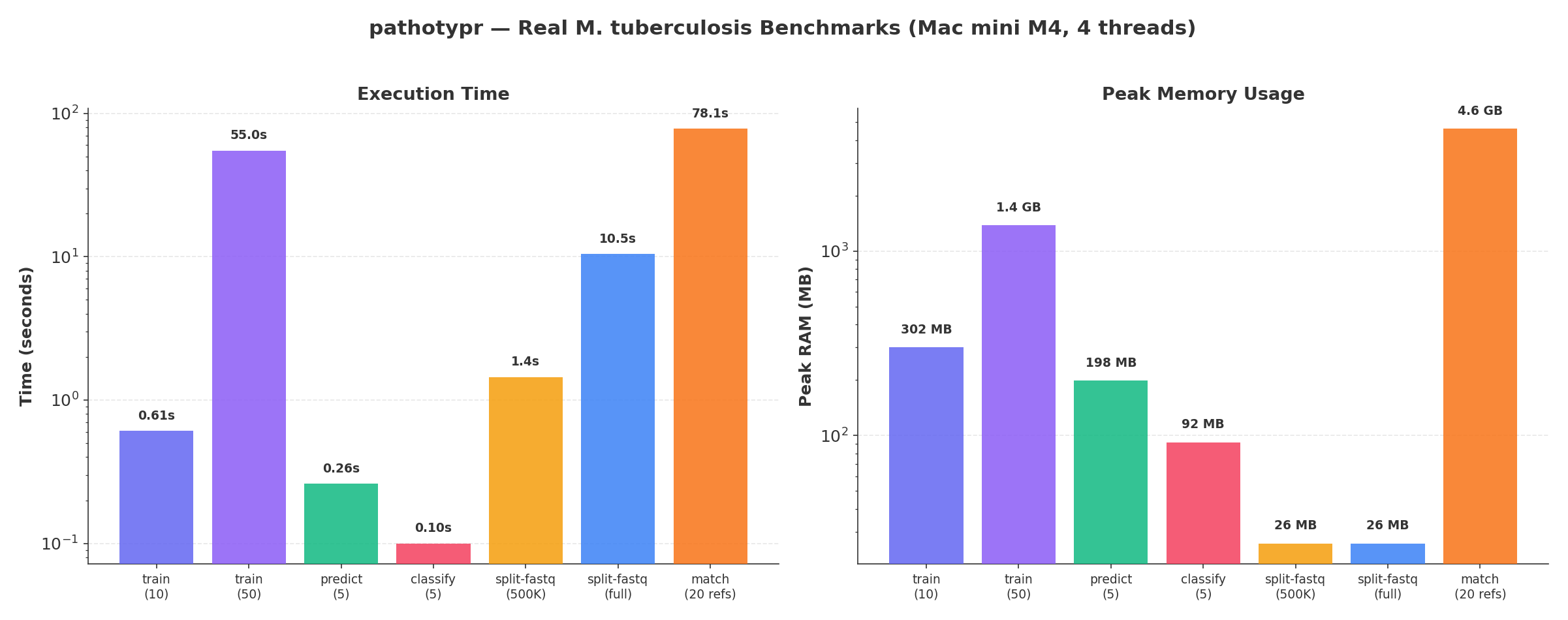
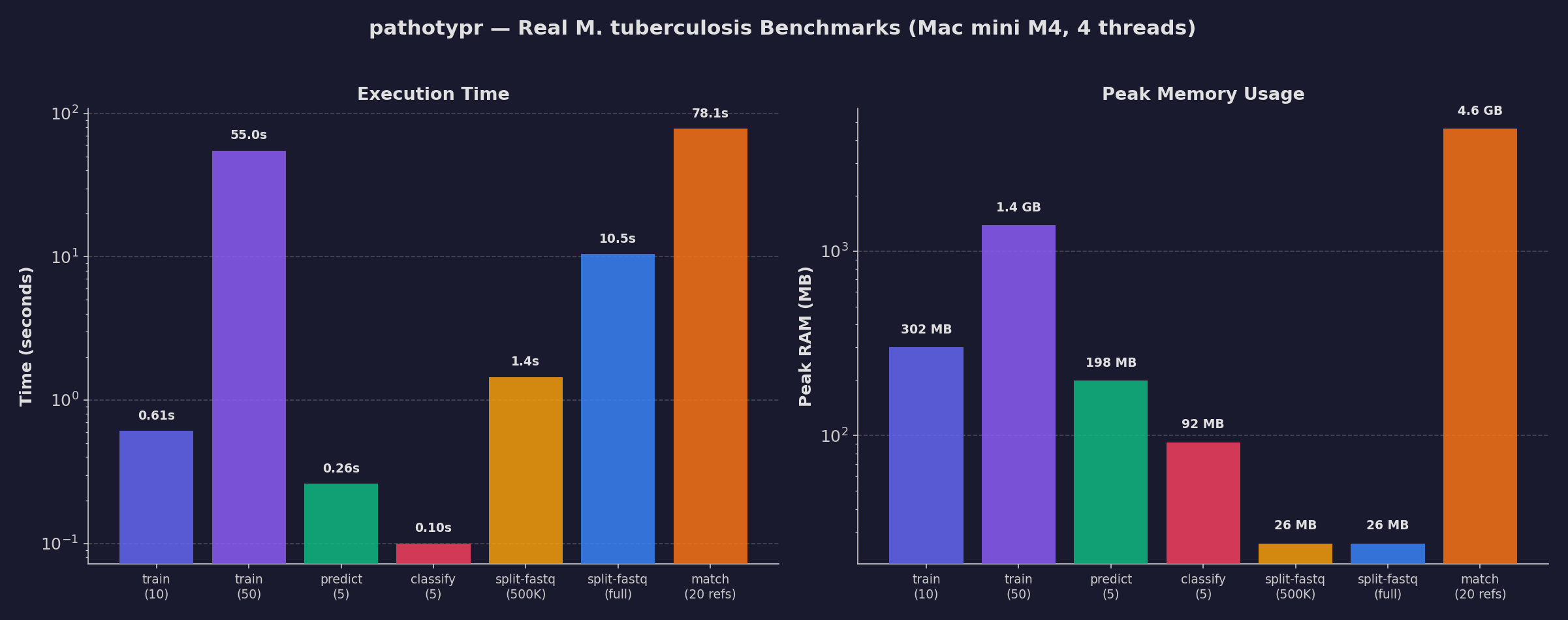
End-to-end benchmarks using real MTB genomes (~4.4 Mb each, k=21) on a Mac mini M4 (4 threads).
Train
| Genomes | Time | Peak RAM | Model Size |
|---|---|---|---|
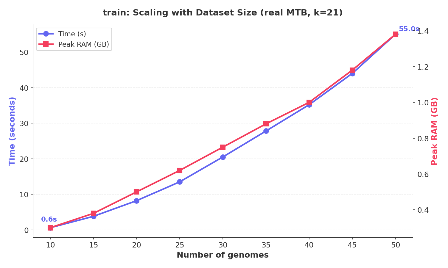
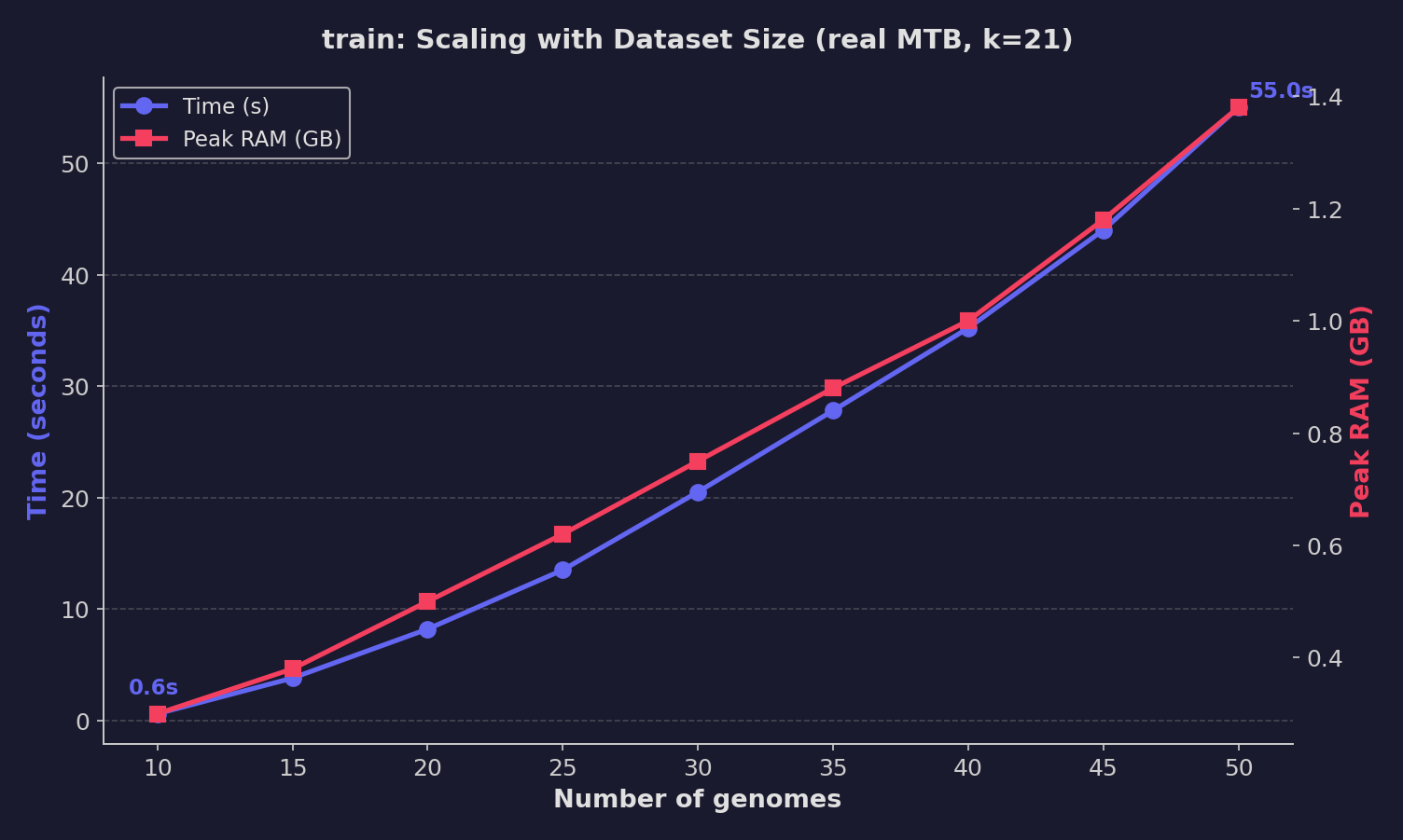
| 10 | 0.6 s | 302 MB | ~13 KB |
| 50 | 55 s | 1,381 MB | ~35 KB |
Training time scales with dataset size due to vectorization (4.4M k-mers per genome) and tree construction.
Predict
| Genomes | Model source | Time | Peak RAM |
|---|---|---|---|
| 5 | 10-genome model | 0.25 s | 197 MB |
| 5 | 50-genome model | 0.26 s | 198 MB |
Prediction is nearly instant (~50 ms/genome), dominated by I/O. Model size has minimal impact on speed.
Classify (Assembly Markers)
| Genomes | Markers | Time | Peak RAM |
|---|---|---|---|
| 5 | 3,707 SNPs | 0.10 s | 92 MB |
Assembly marker calling is extremely fast (~20 ms/genome) — k-mer matching on pre-assembled FASTA.
Split-FASTQ (Read Genotyping)
| Input | Reads | Time | Peak RAM |
|---|---|---|---|
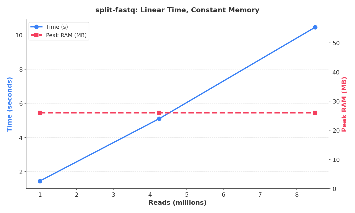
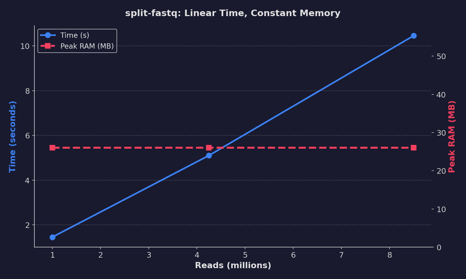
| 500K PE reads (subsampled) | 1M | 1.5 s | 26 MB |
| Full ERR2659157 (65× coverage) | ~8.5M | 10.5 s | 26 MB |
Constant 26 MB memory regardless of input size — Bloom filter + streaming reads. Speed scales linearly with read count.
Match (Reference Matching)
| References | Input | Time | Peak RAM |
|---|---|---|---|
| 20 | 500K PE reads | 78 s | 4,606 MB |
Match is the most memory-intensive module: each reference batch loads ~4.4 Mb genome + ~34 MB k-mer set. Time and memory scale with reference count × read count.
Summary
| Module | Time (typical) | Peak RAM | Scales with |
|---|---|---|---|
| train | 1–60 s | 300–1400 MB | N genomes × genome size |
| predict | 0.25 s | ~200 MB | Input size (streaming) |
| classify | 0.1 s | ~90 MB | N genomes × N markers |
| split-fastq | 1–11 s | 26 MB (constant) | Read count |
| match | 78 s / 20 refs | ~4.6 GB | N references × read count |
Feature comparison with other MTBC tools
Where pathotypr sits next to the tools it is most often compared with.
| pathotypr | fastlin | TB-Profiler | Mykrobe | SNP-IT | KvarQ | |
|---|---|---|---|---|---|---|
| Alignment-free (FASTQ) | ✅ | ✅ | ❌ | ✅ | ❌ | ✅ |
| Assemblies (FASTA) | ✅ | ✅ | ❌ | ❌ | VCF only | ❌ |
| Custom markers | ✅ | ❌ | ❌ | ❌ | ❌ | ❌ |
| ML training | ✅ | ❌ | ❌ | ❌ | ✅ | ❌ |
| DR prediction | ✅ | ❌ | ✅ | ✅ | ❌ | ✅ |
| Desktop GUI | ✅ | ❌ | Web | ✅ | ❌ | ✅ |
| Standalone binary | ✅ | ✅ | ❌ | ❌ | ❌ | ❌ |
| Organism-agnostic | ✅ | TB only | TB only | Limited | TB only | TB only |
| Speed (per sample) | ~1 s | <5 s | 3–10 min | ~3 min | 1–2 min | ~2 min |
Only the pathotypr and fastlin timings below were measured here; the rest of the table reflects each tool's documented capabilities and reported runtimes.
pathotypr vs fastlin — Real TB Data
Head-to-head comparison using real Mycobacterium tuberculosis FASTQ samples from the European Nucleotide Archive.
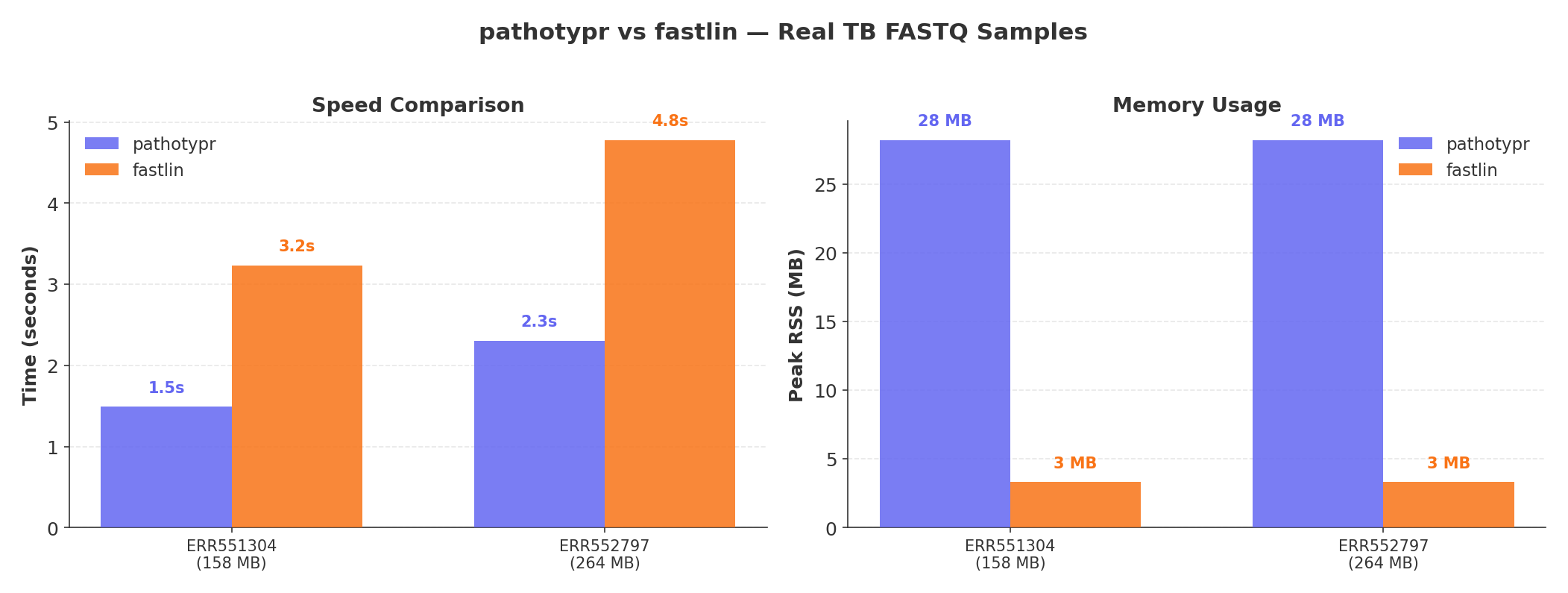
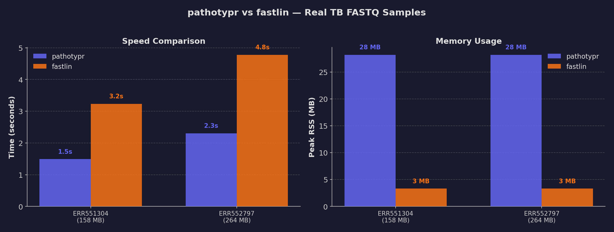
| Sample | FASTQ size | pathotypr | fastlin | Speedup |
|---|---|---|---|---|
| ERR551304 (L2) | 158 MB | 1.49 s | 3.23 s | 2.2× |
| ERR552797 (A4/bovis) | 264 MB | 2.30 s | 4.78 s | 2.1× |
| pathotypr | fastlin | |
|---|---|---|
| Speed | ~2× faster | — |
| Peak RAM | 28 MB | 3 MB |
| Markers | Custom (3,707 SNPs) | Built-in barcodes (1,230) |
| Lineage depth | Full hierarchy (L2;L2.2) | Sub-lineage (2.2.1) |
| Organism | Any (custom markers) | TB only |
Both tools correctly identified the major lineage. pathotypr is consistently ~2× faster due to parallel k-mer scanning with Bloom filter acceleration, while fastlin uses ~10× less memory thanks to its minimal barcode approach.
Test conditions: Mac mini M4, 4 threads, paired-end reads, gzip-compressed FASTQ.
Methodology
- Hardware: Mac mini M4, 16 GB RAM
- Threads: 4 (fixed for reproducibility)
- Sequences: synthetic 1000 bp sequences with class-distinctive k-mer motifs
- Runs: 3 per configuration, median reported
- k-mer size: 11 (smaller than production default of 21, for speed)
- Trees: 100 (production default)
- Peak RSS: measured via
/usr/bin/time -l(macOS)
Scaling expectations for real data
With real bacterial genomes (~4.4 Mb, k=21): - Training 500 genomes: ~10 minutes (extrapolated from 55 s for 50 genomes) - Prediction 500 genomes: ~25 seconds (at the measured ~50 ms/genome) - Model size: tens of KB (13–35 KB measured for 10–50 real MTB genomes)
These benchmarks use small synthetic sequences to isolate algorithmic scaling from I/O. Real-world performance depends on genome size, k-mer size, disk speed, and available cores.