Palettes¶

Three palettes, all exported as plain character vectors of hex codes. Nothing in the package hides them, so they work anywhere a colour vector works, ggplot2 or not:

library(mycolorsTB)

mycolors
classicTB
pathogenomics

Palette	Colours	Names	Reach for it when
`mycolors`	14	lineage identifiers	your categories are MTBC lineages
`classicTB`	the same 14	none	your categories are anything else
`pathogenomics`	8	none	you want the lab's own theme colours

The first two hold exactly the same colours. The only difference is whether they carry names, and that difference decides how a scale built from them matches your data. Matching by name, matching by position is the section to read if you read only one.

mycolors¶

The fourteen lineage colours, named. L1 to L10 are the human-adapted lineages of the Mycobacterium tuberculosis complex and A1 to A4 the animal-adapted ones, which is the labelling most lineage callers emit, so a column of lineage assignments usually matches these names as it stands.

Name	Hex
`A1`	`#d1ae00`
`A2`	`#8ef5c8`
`A3`	`#73c2ff`
`A4`	`#ff9cdb`
`L1`	`#ff3091`
`L2`	`#001aff`
`L3`	`#8a0bd2`
`L4`	`#ff0000`
`L5`	`#995200`
`L6`	`#1eb040`
`L7`	`#fbff00`
`L8`	`#ff9d00`
`L9`	`#37ff30`
`L10`	`#8fbda1`

view_palette("mycolors")

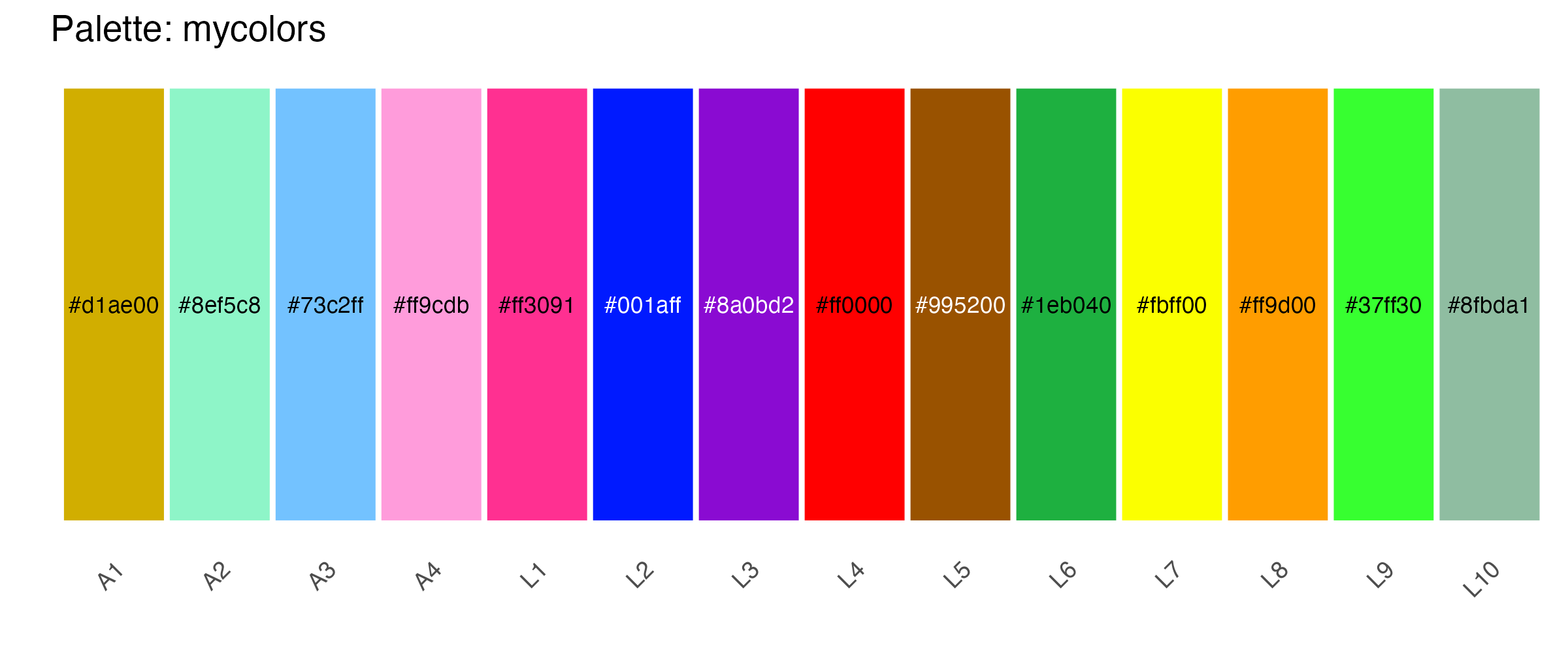
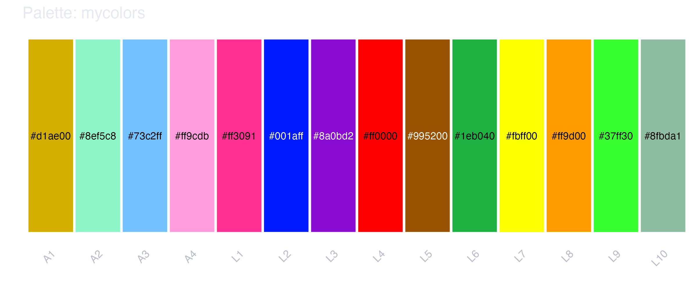
The fourteen mycolors swatches in a row, each labelled with its hex code, under the title Palette: mycolors, with the lineage names as tick labels below

Use it through scale_color_mycolors() and scale_fill_mycolors(), or reach into the vector directly when you need one colour: mycolors["L4"] is L4's red, and mycolors[c("L2", "L4")] is a two-colour vector still carrying its names.

classicTB¶

The same fourteen colours in the same order, with the names taken off:

identical(unname(mycolors), classicTB)
#> TRUE

names(classicTB)
#> NULL

That is the entire difference. classicTB exists so the palette can be used on a categorical variable that has nothing to do with lineages: drug names, sampling sites, clusters, years. Fourteen levels is the ceiling before a scale built from it runs out of colours.

pathogenomics¶

Eight colours from the PathoGenOmics Lab theme. They are not lineage colours and have no lineage meaning: this is the palette for the parts of a figure that are not the data, or for a small categorical variable that should look like it belongs to the lab's other material rather than competing with the lineage colours next to it.

Position	Hex
1	`#c01718`
2	`#305595`
3	`#3c5824`
4	`#d9d0ca`
5	`#9ec4e8`
6	`#c0b3a7`
7	`#fdf2f8`
8	`#020203`

view_palette("pathogenomics")

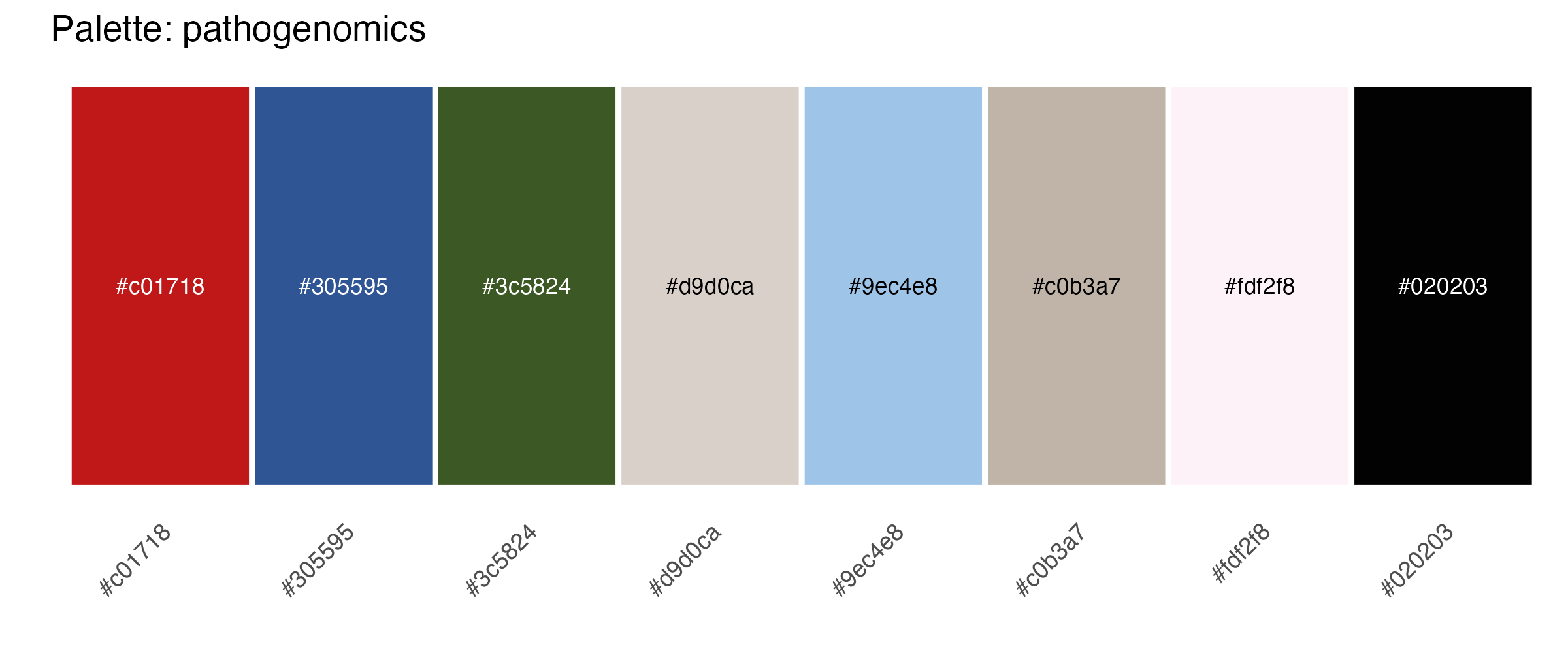
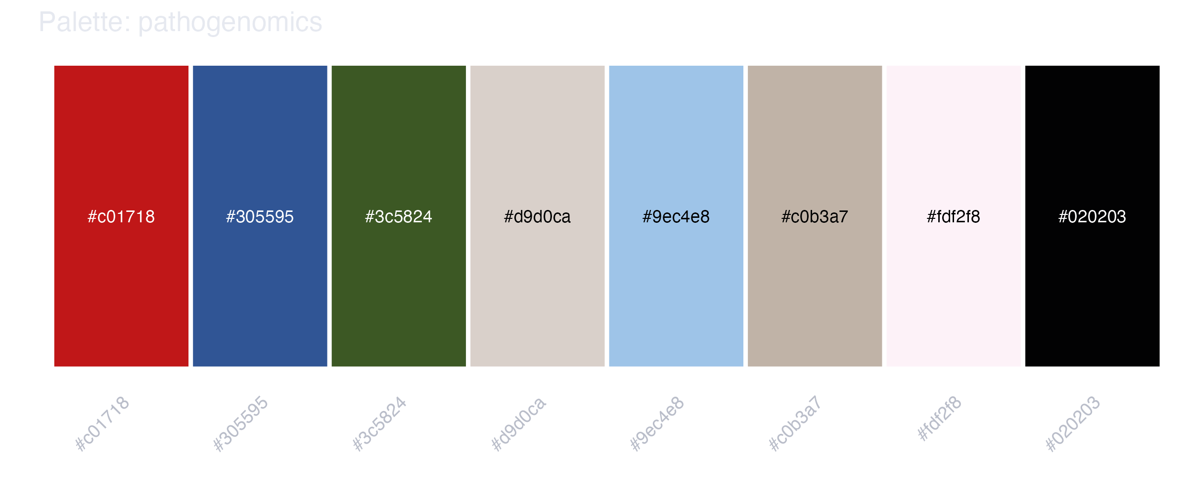
The eight pathogenomics swatches in a row, each labelled with its hex code, with the hex codes repeated as tick labels below because the palette has no names

Note the two ends of it. #fdf2f8 is nearly white and #020203 is nearly black, so whichever end matches your background disappears into it: fill eight shapes with these on a white page and one of them is an outline of nothing. Draw borders, or drop the end you are sitting on.

Matching by name, matching by position¶

This is the one thing about the package that is easy to get wrong, and getting it wrong does not always produce an error.

mycolors matches by name¶

scale_fill_mycolors() passes a named vector to ggplot2::scale_fill_manual(), and a named values vector is matched against the levels of your data by name. A group labelled L4 gets L4's red no matter where it sits in the data, and reordering the bars never moves a colour.

The cost is that a label which is not a lineage name has no colour to match:

library(ggplot2)

counts <- data.frame(
  lineage = c("L1", "L2", "L4", "A1", "L11"),
  isolates = c(41, 58, 96, 3, 7)
)

ggplot(counts, aes(x = lineage, y = isolates, fill = lineage)) +
  geom_col() +
  scale_fill_mycolors(name = "Lineage", na.value = "grey70") +
  labs(x = NULL, y = "Isolates") +
  theme_minimal()

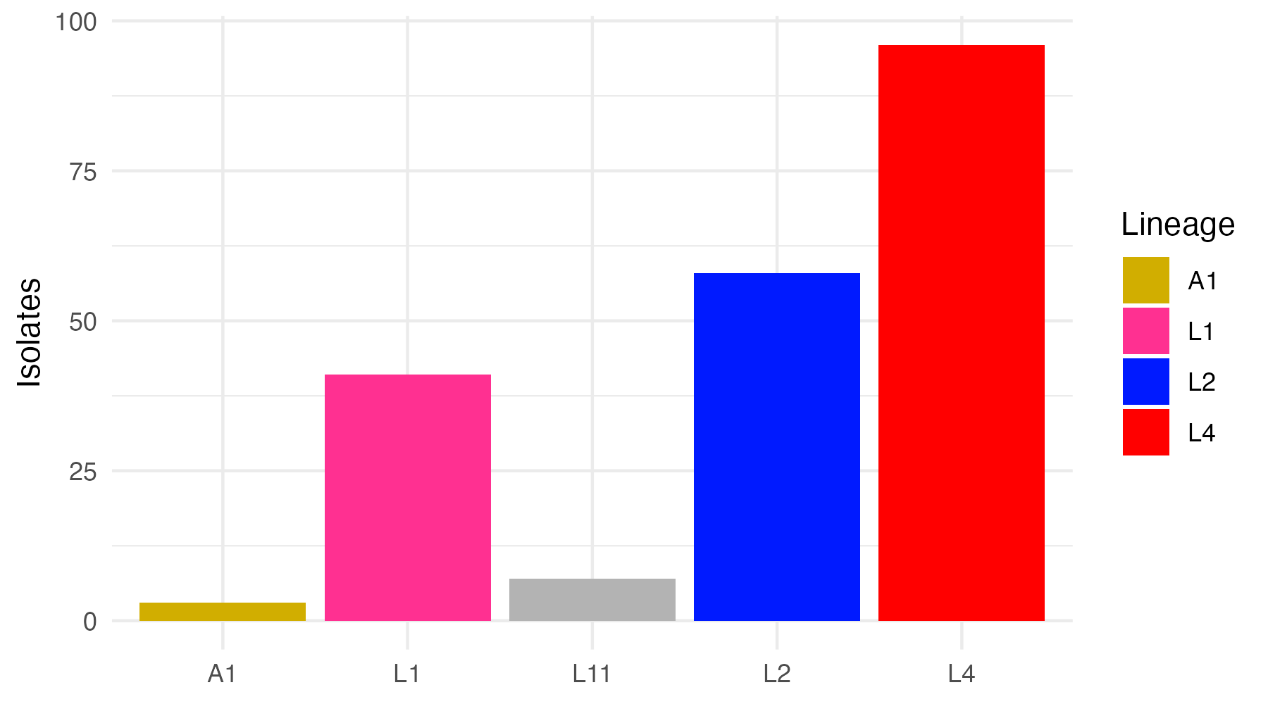
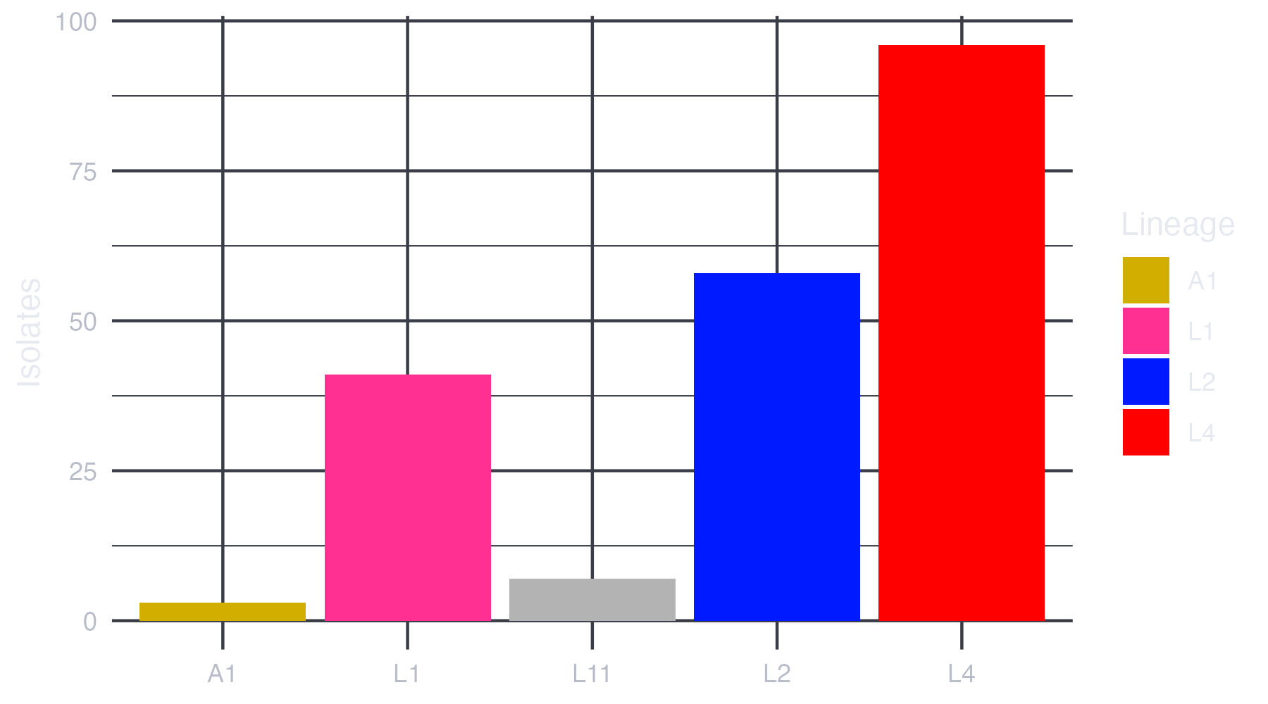
Five bars, four of them in their lineage colours and the L11 bar in grey, with a legend listing only the four matched lineages

L11 is not a name in mycolors, so it takes na.value instead of a colour. Two things about that are worth knowing before it happens to you in a figure you are about to submit:

Nothing warns. The plot builds and prints. Leave na.value unset and the bar comes out ggplot2's default grey50, which looks like a deliberate choice for a missing category rather than a typo in a label.
The unmatched level is not in the legend either. The legend above lists A1, L1, L2 and L4. There is a grey bar on the plot with nothing in the key to explain it.

The one case that does warn is when no level matches at all:

Warning: No shared levels found between `names(values)` of the manual scale and
the data's fill values.

Every shape comes out grey50. That is what you get from pointing scale_fill_mycolors() at a variable of drug names, and it is the signal that you wanted classicTB. ggplot2 scales works through the same ground from the scale functions' side, and Troubleshooting collects the messages.

classicTB matches by position¶

classicTB has no names, so ggplot2 hands the colours out in the order of the scale's levels: first level, first colour.

drugs <- data.frame(
  drug = c("isoniazid", "rifampicin", "ethambutol", "pyrazinamide"),
  resistant = c(112, 88, 34, 51)
)

ggplot(drugs, aes(x = drug, y = resistant, fill = drug)) +
  geom_col() +
  scale_fill_classicTB(name = "Drug") +
  labs(x = NULL, y = "Resistant isolates") +
  theme_minimal()

Anything with up to fourteen levels works, and no label has to mean anything. The cost is the mirror image of the other palette's: the colour a category gets depends on where it falls in the level order, and R sorts character levels alphabetically. Here that is ethambutol, isoniazid, pyrazinamide, rifampicin, so ethambutol takes #d1ae00 and isoniazid, the drug you would have listed first, takes #8ef5c8. Add a fifth drug beginning with a letter before i and every colour after it shifts by one.

If a figure has to keep its colours across a paper, fix the order yourself with factor(drug, levels = c(...)) rather than relying on the alphabet.

Which one do I want

Are the categories lineages, spelled the way mycolors spells them? Use mycolors. Anything else, classicTB.

view_palette()¶

view_palette(palette_name) returns a ggplot of the chosen palette's swatches with each hex code written across its own colour. It takes one of "mycolors", "classicTB" or "pathogenomics", and defaults to "mycolors".

view_palette()
view_palette("classicTB")
view_palette(palette_name = "pathogenomics")

Because it returns a plot object rather than drawing to the device, it composes like any other:

library(ggplot2)

ggsave("mycolors.png", view_palette("mycolors") + labs(title = NULL),
       width = 8, height = 3, dpi = 300)

Two details of what it draws:

Each hex code is written in black or white, chosen from the WCAG relative luminance of its own swatch, so #020203 in pathogenomics reads in white rather than disappearing. On 0.1.1 every label is black and that one is invisible.
For an unnamed palette the tick labels underneath are the hex codes, because there are no names to put there. That is the fastest way to see at a glance which of the three you are looking at.

The palette name is validated, so a near miss stops instead of guessing:

view_palette("mycolours")
#> Error in match.arg(palette_name, choices) :
#>   'arg' should be one of "mycolors", "classicTB", "pathogenomics"

view_palette(1)
#> Error: `palette_name` must be a single palette name, one of: mycolors, classicTB, pathogenomics.

tb_palette()¶

tb_palette(n, palette_name = "classicTB") returns n colours as an unnamed character vector, for the times when you need colours rather than a scale.

While n does not exceed the palette, it returns the palette's own colours, untouched and in order:

tb_palette(5, "classicTB")
#> [1] "#d1ae00" "#8ef5c8" "#73c2ff" "#ff9cdb" "#ff3091"

identical(tb_palette(5, "classicTB"), unname(classicTB[1:5]))
#> [1] TRUE

tb_palette(8, "pathogenomics")
#> [1] "#c01718" "#305595" "#3c5824" "#d9d0ca" "#9ec4e8" "#c0b3a7" "#fdf2f8" "#020203"

Ask for more than the palette holds and it interpolates with grDevices::colorRampPalette(), and says so:

tb_palette(20, "classicTB")
#> Warning: Number of requested colors (20) is greater than the size of the
#> 'classicTB' palette (14). Colors are interpolated.
#>  [1] "#D1AE00" "#A3DE88" "#84E2DC" "#7AC0FD" "#DAA6E4" "#FF6EBB" "#E42D9C"
#>  [8] "#351EE7" "#4112E9" "#9C09B0" "#EC0121" "#C92B00" "#7F650D" "#2AA639"
#> [15] "#9DDD1A" "#FCE500" "#FEA200" "#80DA1E" "#52EA53" "#8FBDA1"

Interpolated colours are not lineage colours

Only the first and last of those twenty are palette colours. #A3DE88 and #84E2DC are points on a ramp between neighbouring palette entries and belong to no lineage at all. tb_palette() returns an unnamed vector in every case, so nothing downstream can tell you which of the colours in your hand still mean something. If the answer has to be a lineage colour, index the palette directly: mycolors[c("L2", "L4")].

This is also where 0.1.1 and 0.1.2 disagree most loudly. On 0.1.1 tb_palette(5, "mycolors") interpolates too, and returns #D1AE00 #FF81C8 #C40569 #C3EB10 #8FBDA1, of which three are not in the palette at all.

Both arguments are checked. n has to be a single non-negative whole number and palette_name a single palette name, so a transposed call fails instead of quietly answering the wrong question:

tb_palette(3, 2)
#> Error: `palette_name` must be a single palette name, one of: mycolors, classicTB, pathogenomics.

tb_palette(-1)
#> Error: `n` must be a single non-negative whole number.

tb_palette(0) is legal and returns character(0).

Colour vision¶

This package is entirely colour. Fourteen categories is a lot to separate by hue alone, and some of these fourteen are close, so it is worth saying what is measured rather than what is hoped.

What was measured. Each of the fourteen mycolors values was passed through colorspace::deutan(), protan() and tritan(), which apply the Machado, Oliveira and Fernandes (2009) simulation of dichromatic vision. All 91 pairs were then compared with farver::compare_colour(method = "cie2000"), the CIEDE2000 difference in CIE Lab. Larger is more distinguishable; the numbers below are that difference, nothing else.

	Normal	Deuteranopia	Protanopia	Tritanopia
Smallest distance in the palette	11.5	2.4	1.5	6.1
Pairs below 10, out of 91	0	7	7	2
Pairs below 5, out of 91	0	1	4	0

With ordinary colour vision the palette holds up: no pair is under 10, and the closest is L2 and L3, the blue and the purple, at 11.5. Under the simulations it does not, and the collapse is not spread evenly. These are the pairs that move furthest:

Pair	Normal	Deuteranopia	Protanopia
`A1` / `L8`	16.6	2.4	1.5
`L8` / `L9`	51.0	6.9	16.3
`L4` / `L6`	75.6	7.0	24.7
`L1` / `L10`	61.9	7.2	34.2
`L7` / `L9`	22.4	8.3	3.7
`L2` / `L3`	11.5	9.7	5.5
`L4` / `L5`	23.4	14.8	1.8
`A2` / `L10`	14.0	11.1	12.6

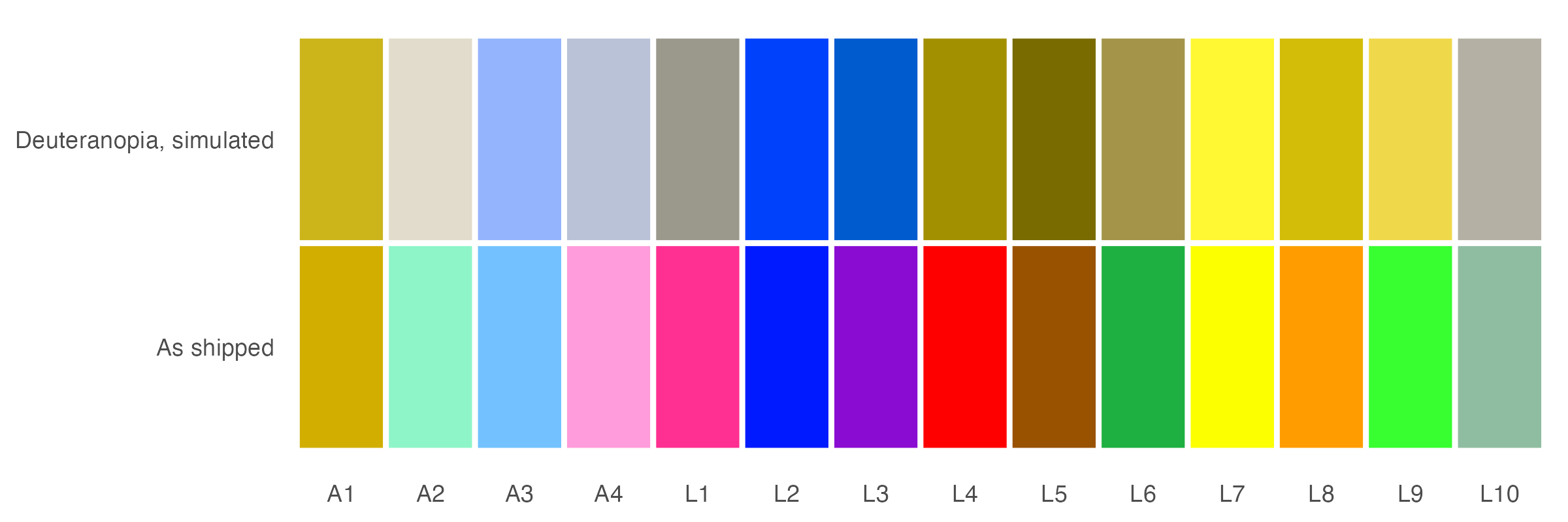
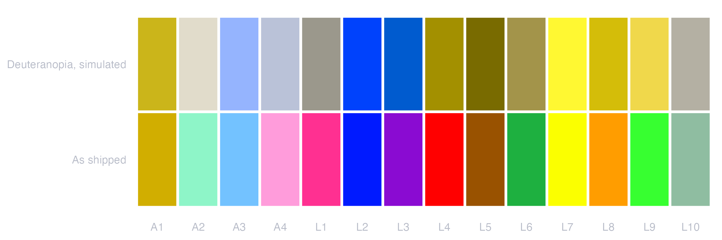
Two rows of fourteen swatches, the lower row the mycolors palette as shipped and the upper row the same colours under a simulation of deuteranopia, in which several distinct colours become the same gold or the same olive

Upper row: the same fourteen colours under colorspace::deutan(). Lower row: the palette as the package ships it.

A1 and L8 are the pair to know about. Gold and orange are already the closest of the warm colours at 16.6, and under either red-green simulation they land on top of each other: #CBB51A and #D4BD09 under deuteranopia, 2.4 apart. The red-green pairs behave the way red-green pairs do, L4 red and L6 green going from 75.6 to 7.0. L2 and L3, the blue and the purple, are the palette's closest pair before any simulation and stay close after one, so they are the pair every reader has to work at.

What follows from that is narrow and practical:

If A1 and L8 are both in the same figure and the reader has to tell them apart, colour will not do it on its own. The same goes for L4 with L6, and for L2 with L3 in every reader.
Most figures do not carry all fourteen. Subsetting the palette to the lineages actually present is the cheapest fix there is, and mycolors[c("L2", "L4", "L6")] is the whole of it.
Where colour has to carry the identity, give it help that is not colour: direct labels, facets, a shape aesthetic. plot_tb_tree() already prints the tip label next to each coloured tip for exactly this reason.

Two honest limits on the numbers above. Dichromacy is the severe end of colour vision deficiency and anomalous trichromacy, which is more common, is milder than these simulations. And a CIEDE2000 distance is a measurement of two patches, not a prediction about a reader looking at a busy figure. Treat the table as a way to find the risky pairs, not as a pass or fail.

Reproduce any of it:

library(mycolorsTB)
library(colorspace)
library(farver)

# Every pairwise CIEDE2000 distance in the palette, before and after a
# simulation of deuteranopia.
distances <- function(hex) {
  lab <- farver::convert_colour(t(grDevices::col2rgb(hex)), "rgb", "lab")
  d <- farver::compare_colour(lab, lab, from_space = "lab", method = "cie2000")
  dimnames(d) <- list(names(mycolors), names(mycolors))
  d
}

normal <- distances(unname(mycolors))
deutan <- distances(colorspace::deutan(unname(mycolors)))

round(c(normal = normal["A1", "L8"], deuteranopia = deutan["A1", "L8"]), 1)
#>       normal deuteranopia
#>         16.6          2.4

colorspace and farver are not dependencies of mycolorsTB. Install them from CRAN if you want to run the block above.

Where to go next¶

ggplot2 scales: the four scale functions in use, and what they forward to ggplot2.
Trees and cladograms: where the lineage names in mycolors stop being a convention and start being a requirement.
Function reference: view_palette(), tb_palette() and the rest, one entry each.
Getting started: installing ggtree from Bioconductor before the package, and telling 0.1.1 from 0.1.2.